![]()
使用 sktime 和 ClaSP 进行时间序列分割#
在本笔记本中,我们将展示如何使用 sktime 和 ClaSP 完成时间序列分割任务。我们将首先介绍时间序列分割的任务,说明 ClaSP 的易用性,并展示一个案例中找到的分割结果。
时间序列分割的任务#
我们将在此笔记本中研究的一个特别有趣的问题是时间序列分割 (TSS)。
TSS 的目标是发现时间序列中与相邻区域语义上不相似的区域。TSS 是一项重要的技术,因为它可以通过分析测量结果来推断底层系统的属性,因为从一个片段到另一个片段的变化通常是由被监控过程中的状态变化引起的,例如从一个操作状态过渡到另一个操作状态,或者异常事件的发生。变点检测 (CPD) 的任务是找到底层信号中的此类变化,而分割则是一系列有序的变点。
下图显示了两个示例:(a) 来自具有不同医疗状况的患者的心跳记录,以及 (b) 一个人走路、慢跑和跑步。时间序列包含三个视觉上非常明显的片段,我们用颜色标注了它们,并用底层状态进行了注释。
任何 TSS 算法的任务都是找到这些片段。
先决条件#
[ ]:
import sys

sys.path.insert(0, "..")

import pandas as pd
import seaborn as sns

sns.set_theme()
sns.set_color_codes()

from sktime.datasets import load_electric_devices_segmentation
from sktime.detection.clasp import ClaSPSegmentation, find_dominant_window_sizes
from sktime.detection.plotting.utils import (
    plot_time_series_with_change_points,
    plot_time_series_with_profiles,
)
以下用例展示了家用电器的能量曲线,其中有四个变点指示了不同的运行状态或已插入的家用电器。
[2]:
ts, period_size, true_cps = load_electric_devices_segmentation()
_ = plot_time_series_with_change_points("Electric Devices", ts, true_cps)
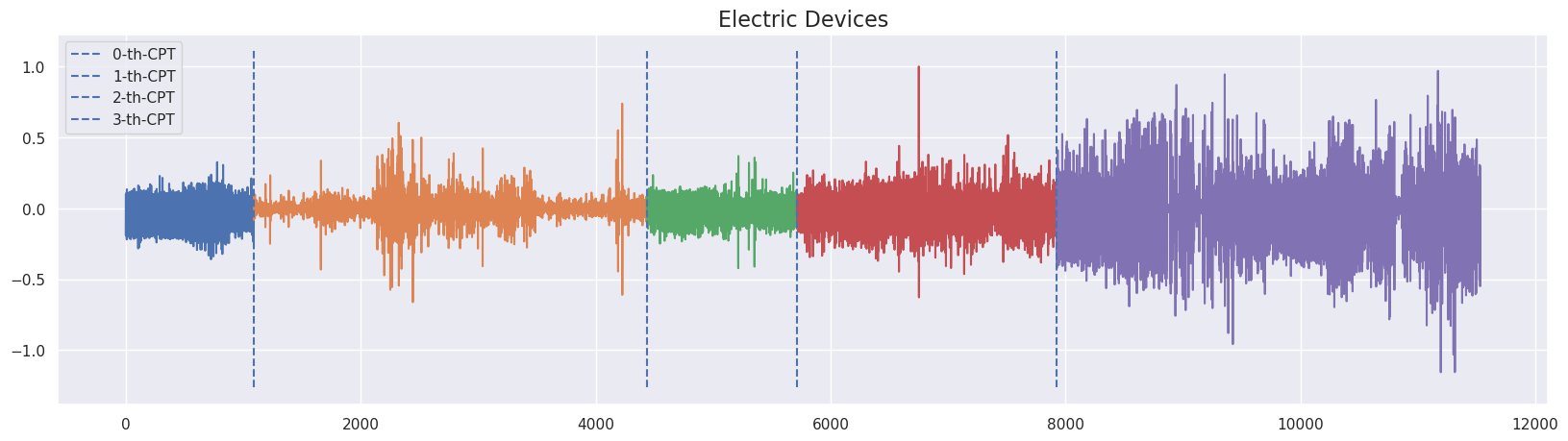
标注的变点大约在时间戳 \([1090,4436,5712,7923]\) 附近,这些变点记录了不同的电器设备。
通过 ClaSP 进行时间序列分割#
本 Jupyter 笔记本演示了如何使用分类分数剖面 (ClaSP) 进行时间序列分割。
ClaSP 将时间序列 (TS) 分层地分成两部分,每个分割点是通过为每个可能的分割点训练一个二元时间序列分类器,并选择准确率最高的那个来确定的,即最擅长识别来自任一分区的子序列的那个分类器。
详情请参考我们发表在 CIKM '21 上的论文:P. Schäfer, A. Ermshaus, U. Leser, ClaSP - Time Series Segmentation, CIKM 2021
获取数据#
首先让我们查看并绘制要分割的时间序列。
[3]:
# ts is a pd.Series
# we convert it into a DataFrame for display purposed only
pd.DataFrame(ts)
[3]:
| 1 | |
|---|---|
| 1 | -0.187086 |
| 2 | 0.098119 |
| 3 | 0.088967 |
| 4 | 0.107328 |
| 5 | -0.193514 |
| ... | ... |
| 11528 | 0.300240 |
| 11529 | 0.200745 |
| 11530 | -0.548908 |
| 11531 | 0.274886 |
| 11532 | 0.274022 |
11532 行 × 1 列
ClaSP - 分类分数剖面#
让我们运行 ClaSP 来找到真实的变点。
ClaSP 有两个超参数
周期长度
要找到的变点数量
ClaSP 的结果是一个剖面,其中的最大值指示了找到的变点。
[4]:
clasp = ClaSPSegmentation(period_length=period_size, n_cps=5)
found_cps = clasp.fit_predict(ts)
profiles = clasp.profiles
scores = clasp.scores
print("The found change points are", found_cps.to_numpy())
The found change points are [1038 4525 5719 7883]
分割可视化#
……然后我们可视化结果。
[5]:
_ = plot_time_series_with_profiles(
    "Electric Devices",
    ts,
    profiles,
    true_cps,
    found_cps,
)
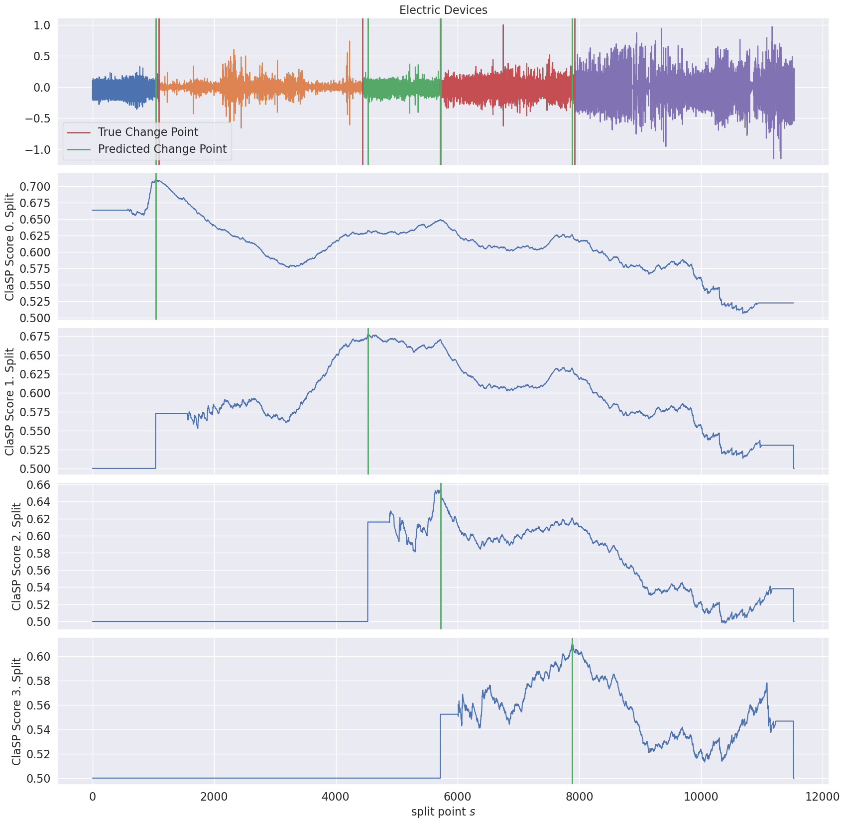
绿色预测的变点与红色真实的变点非常相似。
输出格式#
ClaSP 提供两种不同的输出格式,可以使用 ‘sparse_to_dense’ 或 ‘dense_to_sparse’ 方法访问。
[6]:
clasp = ClaSPSegmentation(period_length=period_size, n_cps=5)
found_segmentation = clasp.fit_predict(ts)
print(found_segmentation)
0    1038
1    4525
2    5719
3    7883
dtype: int64
[7]:
dense_segmentation = clasp.sparse_to_dense(y_sparse=found_segmentation, index=ts.index)
print(dense_segmentation[1035:1040])
print(dense_segmentation[4522:4527])
print(dense_segmentation[5716:5721])
print(dense_segmentation[7880:7885])
1036    0
1037    0
1038    1
1039    0
1040    0
dtype: int64
4523    0
4524    0
4525    1
4526    0
4527    0
dtype: int64
5717    0
5718    0
5719    1
5720    0
5721    0
dtype: int64
7881    0
7882    0
7883    1
7884    0
7885    0
dtype: int64
ClaSP - 窗口大小选择#
ClaSP 将窗口大小 𝑤 作为超参数。此参数对 ClaSP 的性能有数据依赖性影响。选择过小时,所有窗口倾向于看起来相似;选择过大时,窗口有更高的机会与相邻片段重叠,模糊其区分能力。
选择窗口大小的一个简单而有效的方法是傅里叶变换的主导频率。
[8]:
dominant_period_size = find_dominant_window_sizes(ts)
print("Dominant Period", dominant_period_size)
Dominant Period 10
让我们使用找到的主导周期长度来运行 ClaSP。
[9]:
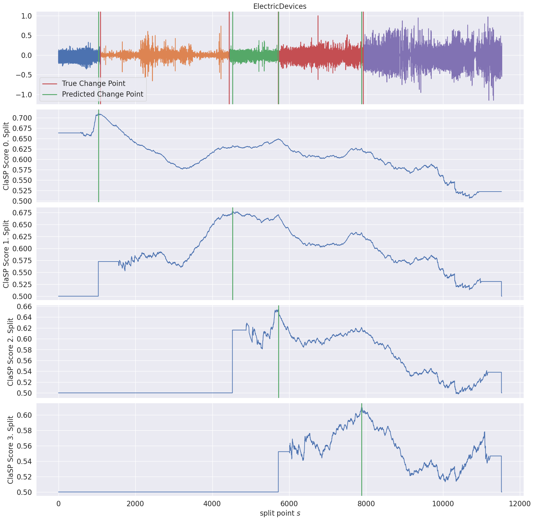
clasp = ClaSPSegmentation(period_length=dominant_period_size, n_cps=5)
found_cps = clasp.fit_predict(ts)
profiles = clasp.profiles
scores = clasp.scores

_ = plot_time_series_with_profiles(
    "ElectricDevices",
    ts,
    profiles,
    true_cps,
    found_cps,
)