![]()
使用 sktime 进行层级、面板和全局预测#
本 notebook 概述#
介绍 - 层级时间序列
sktime 中的层级和面板数据格式
预测器和 Transformer 的自动化向量化
sktime 中的层级协调
使用汇总/缩减模型进行层级预测/全局预测,“M5 获胜者”
扩展器指南
介绍 - 全局预测
不使用外部数据进行全局预测
使用外部数据进行全局预测
贡献者致谢
[1]:
%%capture
import warnings

warnings.filterwarnings("ignore")
层级时间序列#
时间序列通常以“层级”形式呈现,例如
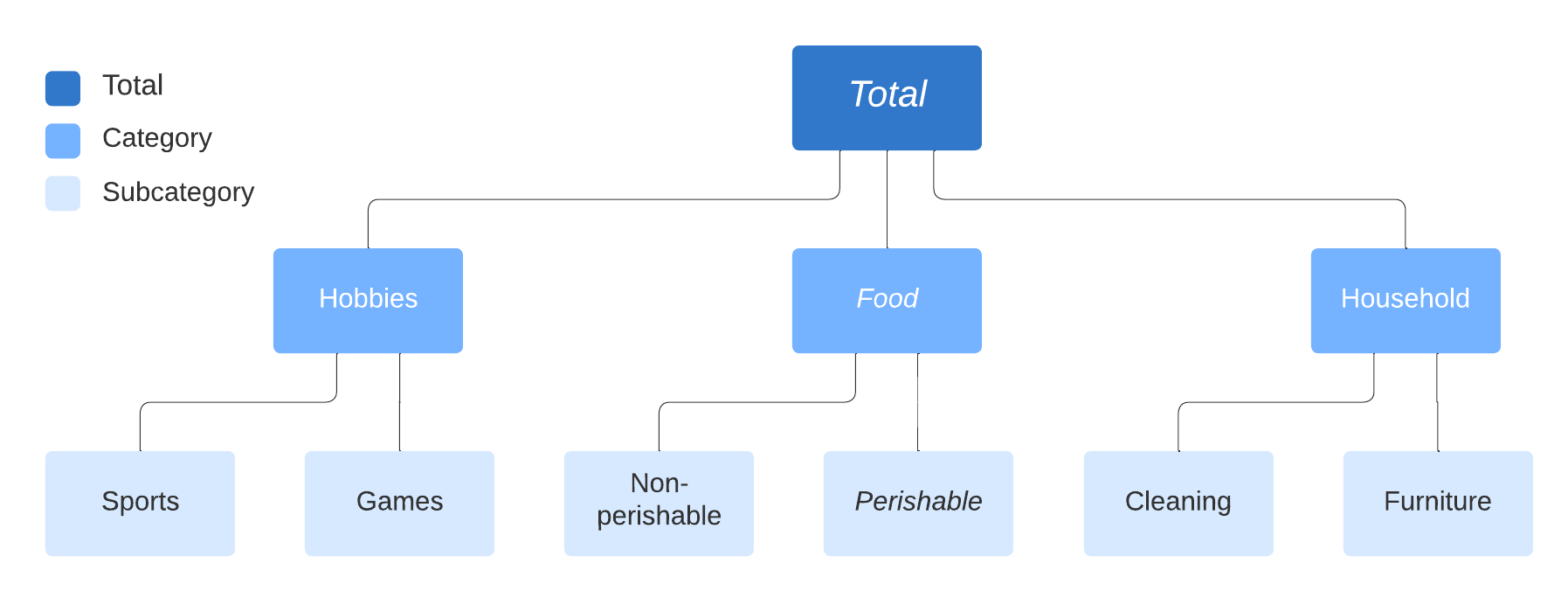
示例包括
不同类别的产品销售(例如 M5 时间序列竞赛)
不同地区的旅游需求
不同成本中心/账户的资产负债表结构
许多层级时间序列数据集可以在这里找到:https://forecastingdata.org/(访问加载器正在开发中)
相关文献请参阅:https://otexts.com/fpp2/hierarchical.html
时间序列也可以展现多个独立的层级结构
层级和面板数据类型的表示#
sktime 将时间序列区分抽象科学数据类型(即“scitypes”)
Series类型 = 一个时间序列(单变量或多变量)Panel类型 = 多个时间序列的集合,扁平层级Hierarchical类型 = 时间序列的层级集合,如上所述
每个 scitype 都有多种 mtype 表示形式。
为简单起见,下面我们只关注基于 pandas.DataFrame 的表示形式。
[2]:
# import to retrieve examples

from sktime.datatypes import get_examples
在 "pd.DataFrame" mtype 中,时间序列由内存容器 obj: pandas.DataFrame 表示,如下所示。
结构约定:
obj.index必须是单调的,并且是Int64Index,RangeIndex,DatetimeIndex,PeriodIndex之一。变量:
obj的列对应于不同的变量变量名:列名
obj.columns时间点:
obj的行对应于不同、离散的时间点时间索引:
obj.index被解释为时间索引。能力:可以表示多变量时间序列;可以表示非等间隔时间序列
"pd.DataFrame" 表示形式中的示例。"a" 和 "b"。两者都在相同的时间点 0, 1, 2, 3 被观测。[3]:
get_examples(mtype="pd.DataFrame")[0]
[3]:
| a | |
|---|---|
| 0 | 1.0 |
| 1 | 4.0 |
| 2 | 0.5 |
| 3 | -3.0 |
"pd.DataFrame" 表示形式中的示例。"a" 和 "b"。两者都在相同的时间点 0, 1, 2, 3 被观测。[4]:
get_examples(mtype="pd.DataFrame")[1]
[4]:
| a | b | |
|---|---|---|
| 0 | 1.0 | 3.000000 |
| 1 | 4.0 | 7.000000 |
| 2 | 0.5 | 2.000000 |
| 3 | -3.0 | -0.428571 |
在 "pd-multiindex" mtype 中,时间序列面板由内存容器 obj: pandas.DataFrame 表示,如下所示。
结构约定:
obj.index必须是类型为(RangeIndex, t)的二元多重索引,其中t是Int64Index,RangeIndex,DatetimeIndex,PeriodIndex之一且单调。实例:具有相同
"instances"索引的行对应于同一实例;具有不同"instances"索引的行对应于不同实例。实例索引:
obj.index中对的第一个元素被解释为实例索引。变量:
obj的列对应于不同的变量变量名:列名
obj.columns时间点:
obj中具有相同"timepoints"索引的行对应于同一时间点;具有不同"timepoints"索引的行对应于不同的时间点。时间索引:
obj.index中对的第二个元素被解释为时间索引。能力:可以表示多变量时间序列的面板;可以表示非等间隔时间序列;可以表示支持时间点不同的面板;不能表示具有不同变量集的时间序列面板。
多变量时间序列面板在 "pd-multiindex" mtype 表示形式中的示例。该面板包含三个多变量时间序列,实例索引为 0, 1, 2。所有时间序列都有两个变量,名称分别为 "var_0", "var_1"。所有时间序列都在三个时间点 0, 1, 2 被观测。
[5]:
get_examples(mtype="pd-multiindex")[0]
[5]:
| var_0 | var_1 | ||
|---|---|---|---|
| 实例 | 时间点 | ||
| 0 | 0 | 1 | 4 |
| 1 | 2 | 5 | |
| 2 | 3 | 6 | |
| 1 | 0 | 1 | 4 |
| 1 | 2 | 55 | |
| 2 | 3 | 6 | |
| 2 | 0 | 1 | 42 |
| 1 | 2 | 5 | |
| 2 | 3 | 6 |
结构约定:
obj.index必须是 3 层或更多层的多重索引,类型为(RangeIndex, ..., RangeIndex, t),其中t是Int64Index,RangeIndex,DatetimeIndex,PeriodIndex之一且单调。我们将最后一个索引称为“时间类”索引层级级别:具有相同非时间类索引的行对应于同一层级单元;具有不同非时间类索引组合的行对应于不同层级单元。
层级:
obj.index中的非时间类索引被解释为层级标识索引。变量:
obj的列对应于不同的变量变量名:列名
obj.columns时间点:
obj中具有相同"timepoints"索引的行对应于同一时间点;具有不同"timepoints"索引的行对应于不同的时间点。时间索引:
obj.index中元组的最后一个元素被解释为时间索引。能力:可以表示层级时间序列;可以表示非等间隔时间序列;可以表示支持时间点不同的层级时间序列;不能表示具有不同变量集的层级时间序列。
[6]:
X = get_examples(mtype="pd_multiindex_hier")[0]
X
[6]:
| var_0 | var_1 | |||
|---|---|---|---|---|
| foo | bar | 时间点 | ||
| a | 0 | 0 | 1 | 4 |
| 1 | 2 | 5 | ||
| 2 | 3 | 6 | ||
| 1 | 0 | 1 | 4 | |
| 1 | 2 | 55 | ||
| 2 | 3 | 6 | ||
| 2 | 0 | 1 | 42 | |
| 1 | 2 | 5 | ||
| 2 | 3 | 6 | ||
| b | 0 | 0 | 1 | 4 |
| 1 | 2 | 5 | ||
| 2 | 3 | 6 | ||
| 1 | 0 | 1 | 4 | |
| 1 | 2 | 55 | ||
| 2 | 3 | 6 | ||
| 2 | 0 | 1 | 42 | |
| 1 | 2 | 5 | ||
| 2 | 3 | 6 |
[7]:
X.index.get_level_values(level=-1)
Int64Index([0, 1, 2, 0, 1, 2, 0, 1, 2, 0, 1, 2, 0, 1, 2, 0, 1, 2], dtype='int64', name='timepoints')
预测器和 Transformer 的自动化向量化(类型转换)#
许多 Transformer 和预测器是为单个时间序列实现的
sktime 会自动将它们向量化/“向上转换”为层级数据
“在层级结构中按个体时间序列/面板应用”
构建层级时间序列
[8]:
from sktime.utils._testing.hierarchical import _make_hierarchical

y = _make_hierarchical()
y
[8]:
| c0 | |||
|---|---|---|---|
| h0 | h1 | time | |
| h0_0 | h1_0 | 2000-01-01 | 1.954666 |
| 2000-01-02 | 4.749032 | ||
| 2000-01-03 | 3.116761 | ||
| 2000-01-04 | 3.951981 | ||
| 2000-01-05 | 3.789698 | ||
| ... | ... | ... | ... |
| h0_1 | h1_3 | 2000-01-08 | 2.044946 |
| 2000-01-09 | 2.609192 | ||
| 2000-01-10 | 4.107474 | ||
| 2000-01-11 | 3.194098 | ||
| 2000-01-12 | 3.712494 |
96 行 × 1 列
[9]:
from sktime.forecasting.arima import ARIMA

forecaster = ARIMA()

y_pred = forecaster.fit(y, fh=[1, 2]).predict()
y_pred
[9]:
| c0 | |||
|---|---|---|---|
| h0 | h1 | ||
| h0_0 | h1_0 | 2000-01-13 | 2.972898 |
| 2000-01-14 | 2.990252 | ||
| h1_1 | 2000-01-13 | 3.108714 | |
| 2000-01-14 | 3.641990 | ||
| h1_2 | 2000-01-13 | 3.263830 | |
| 2000-01-14 | 3.040534 | ||
| h1_3 | 2000-01-13 | 3.186436 | |
| 2000-01-14 | 3.031391 | ||
| h0_1 | h1_0 | 2000-01-13 | 2.483968 |
| 2000-01-14 | 2.568648 | ||
| h1_1 | 2000-01-13 | 2.583254 | |
| 2000-01-14 | 2.591526 | ||
| h1_2 | 2000-01-13 | 3.114990 | |
| 2000-01-14 | 3.078702 | ||
| h1_3 | 2000-01-13 | 2.979505 | |
| 2000-01-14 | 3.029302 |
forecasters_ 属性中pandas.DataFrametransformers_)[10]:
forecaster.forecasters_
[10]:
| 预测器 | ||
|---|---|---|
| h0 | h1 | |
| h0_0 | h1_0 | ARIMA() |
| h1_1 | ARIMA() | |
| h1_2 | ARIMA() | |
| h1_3 | ARIMA() | |
| h0_1 | h1_0 | ARIMA() |
| h1_1 | ARIMA() | |
| h1_2 | ARIMA() | |
| h1_3 | ARIMA() |
要访问或检查个体预测器,请访问 forecasters_ 数据帧的元素
[11]:
forecaster.forecasters_.iloc[0, 0].summary()
[11]:
| 因变量 | y | 观测数量 | 12 |
|---|---|---|---|
| 模型 | SARIMAX(1, 0, 0) | 对数似然 | -15.852 |
| 日期 | 周一, 2022 年 4 月 11 日 | AIC | 37.704 |
| 时间 | 06:55:46 | BIC | 39.159 |
| 样本 | 0 | HQIC | 37.165 |
| - 12 | |||
| 协方差类型 | opg |
| 系数 | 标准误差 | z | P>|z| | [0.025 | 0.975] | |
|---|---|---|---|---|---|---|
| 截距 | 2.9242 | 1.285 | 2.275 | 0.023 | 0.405 | 5.443 |
| ar.L1 | 0.0222 | 0.435 | 0.051 | 0.959 | -0.831 | 0.876 |
| sigma2 | 0.8221 | 0.676 | 1.217 | 0.224 | -0.502 | 2.146 |
| Ljung-Box (L1) (Q) | 0.00 | Jarque-Bera (JB) | 1.13 |
|---|---|---|---|
| Prob(Q) | 0.99 | Prob(JB) | 0.57 |
| 异方差性 (H) | 0.52 | 偏度 | 0.55 |
| Prob(H) (双侧) | 0.55 | 峰度 | 1.98 |
警告
[1] 使用梯度的外积(复数步长)计算协方差矩阵。
对于概率预测也会进行自动向量化(参见 notebook 2)
[12]:
forecaster.predict_interval()
[12]:
| 覆盖范围 | ||||
|---|---|---|---|---|
| 0.9 | ||||
| 下限 | 上限 | |||
| h0 | h1 | |||
| h0_0 | h1_0 | 2000-01-13 | 1.481552 | 4.464243 |
| 2000-01-14 | 1.498538 | 4.481966 | ||
| h1_1 | 2000-01-13 | 1.807990 | 4.409437 | |
| 2000-01-14 | 2.247328 | 5.036651 | ||
| h1_2 | 2000-01-13 | 1.630340 | 4.897320 | |
| 2000-01-14 | 1.378545 | 4.702523 | ||
| h1_3 | 2000-01-13 | 2.001023 | 4.371850 | |
| 2000-01-14 | 1.785088 | 4.277694 | ||
| h0_1 | h1_0 | 2000-01-13 | 1.057036 | 3.910900 |
| 2000-01-14 | 1.121161 | 4.016136 | ||
| h1_1 | 2000-01-13 | 1.825167 | 3.341341 | |
| 2000-01-14 | 1.818342 | 3.364710 | ||
| h1_2 | 2000-01-13 | 1.521553 | 4.708427 | |
| 2000-01-14 | 1.484741 | 4.672664 | ||
| h1_3 | 2000-01-13 | 1.826515 | 4.132494 | |
| 2000-01-14 | 1.873655 | 4.184949 | ||
预测器/原生实现哪个级别以及何时进行向量化取决于“内部 mtype”属性。
对于预测器,检查 y_inner_mtype,这是一个内部支持的机器类型列表
[13]:
forecaster.get_tag("y_inner_mtype")
[13]:
'pd.Series'
Series 级别的 mtype。有关所有 mtype 代码及其对应的 scitype(时间序列、面板或层级)的注册表,sktime.datatypes.MTYPE_REGISTER(转换为 pandas.DataFrame 以获得美观的打印输出)[14]:
import pandas as pd

from sktime.datatypes import MTYPE_REGISTER

pd.DataFrame(MTYPE_REGISTER)
[14]:
| 0 | 1 | 2 | |
|---|---|---|---|
| 0 | pd.Series | Series | 单变量时间序列的 pd.Series 表示 |
| 1 | pd.DataFrame | Series | 单变量或多变量时间序列的 pd.DataFrame 表示... |
| 2 | np.ndarray | Series | 二维 numpy.ndarray,行=样本,列=变量... |
| 3 | nested_univ | Panel | pd.DataFrame,每变量一列,pd.... (似乎被截断了) |
| 4 | numpy3D | Panel | 三维 np.array,格式 (n_instances, n_columns,... (似乎被截断了) |
| 5 | numpyflat | Panel | 警告:仅供内部使用,非完全支持... |
| 6 | pd-multiindex | Panel | 带有多重索引 (instances, time...) 的 pd.DataFrame (似乎被截断了) |
| 7 | pd-wide | Panel | 宽格式的 pd.DataFrame,列 = (instance*... (似乎被截断了) |
| 8 | pd-long | Panel | 长格式的 pd.DataFrame,列 = (index, ti... (似乎被截断了) |
| 9 | df-list | Panel | pd.DataFrame 列表 |
| 10 | pd_multiindex_hier | Hierarchical | 带有 MultiIndex 的 pd.DataFrame |
| 11 | alignment | Alignment | 对齐格式的 pd.DataFrame,值是 i... (似乎被截断了) |
| 12 | alignment_loc | Alignment | 对齐格式的 pd.DataFrame,值是 l... (似乎被截断了) |
| 13 | pd_DataFrame_Table | Table | 数据表的 pd.DataFrame 表示 |
| 14 | numpy1D | Table | 单变量表的 1D np.narray 表示 |
| 15 | numpy2D | Table | 单变量表的 2D np.narray 表示 |
| 16 | pd_Series_Table | Table | 数据表的 pd.Series 表示 |
| 17 | list_of_dict | Table | 包含原始条目的字典列表 |
| 18 | pred_interval | Proba | 预测区间 |
| 19 | pred_quantiles | Proba | 分位数预测 |
| 20 | pred_var | Proba | 方差预测 |
路线图项
使用原生层级支持对接和实现常用方法
使用层级因素的 ARIMA,GEE,混合效应模型
将“使用层级级别”作为协变量或外部特征的包装器
对变量进行完全向量化,使单变量预测器成为多变量预测器
欢迎贡献!
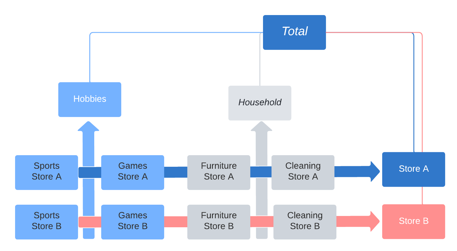
层级协调#
自下而上协调 的工作方式是只在最低层级生成预测,然后向上汇总到所有更高级别的总计。
* Arguably the most simple of all algorithms to reconcile across hierarchies.
* Advantages: easy to implement
* Disadvantages: lower levels of hierarchy are prone to excess volatility. This excess volatility is aggregated up, often producing much less accurate top level forecasts.
自上而下协调 的工作方式是生成最高层级的预测,然后根据较低层级的相对比例等将其分解到最低层级。
* Advantages: still easy to implement, top level is stable
* Disadvantages: peculiarities of lower levels of hierarchy ignored
最优预测协调 的工作方式是在层级结构的所有层级生成预测,并以最小化预测误差的方式调整所有预测结果
* Advantages: often found to be most accurate implementation
* Disadvantages: more difficult to implement
sktime 提供了协调功能
节点级聚合的数据容器约定
计算节点级聚合的功能 -
Aggregator可用于自下而上协调
实现协调逻辑的 Transformer -
Reconciler实现自上而下协调
实现类似 Transformer 的最优预测协调
sktime 使用 pd_multiindex_hier 格式的一个特例来存储节点级聚合
实例(非时间类)级别中的
__total索引元素表示对该级别以下所有实例进行求和__total索引元素是保留的,不能用于其他目的在找到
__total元素的同一级别中,位于__total索引元素下的条目是对所有其他实例条目求和的结果
通过应用 Aggregator Transformer,可以获得节点级聚合格式。
在非聚合输入的管道中,这允许按总计进行预测。
[15]:
from sktime.datatypes import get_examples

y_hier = get_examples("pd_multiindex_hier")[1]
y_hier
[15]:
| var_0 | |||
|---|---|---|---|
| foo | bar | 时间点 | |
| a | 0 | 0 | 1 |
| 1 | 2 | ||
| 2 | 3 | ||
| 1 | 0 | 1 | |
| 1 | 2 | ||
| 2 | 3 | ||
| 2 | 0 | 1 | |
| 1 | 2 | ||
| 2 | 3 | ||
| b | 0 | 0 | 1 |
| 1 | 2 | ||
| 2 | 3 | ||
| 1 | 0 | 1 | |
| 1 | 2 | ||
| 2 | 3 | ||
| 2 | 0 | 1 | |
| 1 | 2 | ||
| 2 | 3 |
[16]:
from sktime.transformations.hierarchical.aggregate import Aggregator

Aggregator().fit_transform(y_hier)
[16]:
| var_0 | |||
|---|---|---|---|
| foo | bar | 时间点 | |
| __total | __total | 0 | 6 |
| 1 | 12 | ||
| 2 | 18 | ||
| a | 0 | 0 | 1 |
| 1 | 2 | ||
| 2 | 3 | ||
| 1 | 0 | 1 | |
| 1 | 2 | ||
| 2 | 3 | ||
| 2 | 0 | 1 | |
| 1 | 2 | ||
| 2 | 3 | ||
| __total | 0 | 3 | |
| 1 | 6 | ||
| 2 | 9 | ||
| b | 0 | 0 | 1 |
| 1 | 2 | ||
| 2 | 3 | ||
| 1 | 0 | 1 | |
| 1 | 2 | ||
| 2 | 3 | ||
| 2 | 0 | 1 | |
| 1 | 2 | ||
| 2 | 3 | ||
| __total | 0 | 3 | |
| 1 | 6 | ||
| 2 | 9 |
如果在管道开始时使用,则对 __total 节点和个体实例都进行预测。
注意:通常情况下,这不会得到协调的预测结果,即预测总计不会相加一致。
[17]:
from sktime.forecasting.naive import NaiveForecaster

pipeline_to_forecast_totals = Aggregator() * NaiveForecaster()

pipeline_to_forecast_totals.fit(y_hier, fh=[1, 2])
pipeline_to_forecast_totals.predict()
[17]:
| 0 | |||
|---|---|---|---|
| foo | bar | ||
| __total | __total | 3 | 18 |
| 4 | 18 | ||
| a | 0 | 3 | 3 |
| 4 | 3 | ||
| 1 | 3 | 3 | |
| 4 | 3 | ||
| 2 | 3 | 3 | |
| 4 | 3 | ||
| __total | 3 | 9 | |
| 4 | 9 | ||
| b | 0 | 3 | 3 |
| 4 | 3 | ||
| 1 | 3 | 3 | |
| 4 | 3 | ||
| 2 | 3 | 3 | |
| 4 | 3 | ||
| __total | 3 | 9 | |
| 4 | 9 |
如果在管道结束时使用,则预测会自下而上协调。
这将得到协调的预测结果,尽管自下而上可能不是首选方法。
[18]:
from sktime.forecasting.naive import NaiveForecaster

pipeline_to_forecast_totals = NaiveForecaster() * Aggregator()

pipeline_to_forecast_totals.fit(y_hier, fh=[1, 2])
pipeline_to_forecast_totals.predict()
[18]:
| 0 | |||
|---|---|---|---|
| foo | bar | ||
| __total | __total | 3 | 18 |
| 4 | 18 | ||
| a | 0 | 3 | 3 |
| 4 | 3 | ||
| 1 | 3 | 3 | |
| 4 | 3 | ||
| 2 | 3 | 3 | |
| 4 | 3 | ||
| __total | 3 | 9 | |
| 4 | 9 | ||
| b | 0 | 3 | 3 |
| 4 | 3 | ||
| 1 | 3 | 3 | |
| 4 | 3 | ||
| 2 | 3 | 3 | |
| 4 | 3 | ||
| __total | 3 | 9 | |
| 4 | 9 |
对于类似 Transformer 的协调,请使用 Reconciler。它支持 OLS 和 WLS 等高级技术
[19]:
from sktime.transformations.hierarchical.reconcile import Reconciler

pipeline_with_reconciliation = (
    Aggregator() * NaiveForecaster() * Reconciler(method="ols")
)
[20]:
pipeline_to_forecast_totals.fit(y_hier, fh=[1, 2])
pipeline_to_forecast_totals.predict()
[20]:
| 0 | |||
|---|---|---|---|
| foo | bar | ||
| __total | __total | 3 | 18 |
| 4 | 18 | ||
| a | 0 | 3 | 3 |
| 4 | 3 | ||
| 1 | 3 | 3 | |
| 4 | 3 | ||
| 2 | 3 | 3 | |
| 4 | 3 | ||
| __total | 3 | 9 | |
| 4 | 9 | ||
| b | 0 | 3 | 3 |
| 4 | 3 | ||
| 1 | 3 | 3 | |
| 4 | 3 | ||
| 2 | 3 | 3 | |
| 4 | 3 | ||
| __total | 3 | 9 | |
| 4 | 9 |
路线图项
包装器类型的协调
协调与全局预测
概率协调
sktime 中的全局预测#
全局预测/面板预测 - 介绍#
也称为
“面板预测”,如果预测所有时间序列
“交叉学习”,如果训练时间序列与部署集不相交
为什么全局预测很重要?
在实践中,我们经常有范围有限的时间序列
估计困难,且无法建模复杂的依赖关系
全局预测的假设:我们可以多次观测到相同的数据生成过程 (DGP)
非相同的 DGP 也可以,只要异同程度能够通过外部信息捕获
现在我们拥有更多信息,可以更可靠地估计更复杂的模型(注意:除非复杂性完全由时间动态驱动)
由于这些优势,全局预测模型在竞赛中非常成功,例如
Rossmann 商店销售
沃尔玛恶劣天气下的销售
M5 竞赛
实践中的许多业务问题本质上都是全局预测问题 - 通常也反映了层级信息(参见上文)
不同类别的产品销售(例如 M5 时间序列竞赛)
不同成本中心/账户的资产负债表结构
在不同时间点观测到的流行病动态
与多变量预测的区别
多变量预测侧重于建模时间序列之间的相互依赖性
全局预测可以建模相互依赖性,但重点在于增强观测空间
sktime 中的实现
所有模型都支持面板预测 - 这些预测可以是独立的或相关的
一些模型的面板预测使用所有时间序列,例如,缩减预测器
可以在不相交示例上训练(“交叉学习”)的模型具有
capability:global_forecasting标签
使用缩减预测器进行面板预测#
对于以下示例,我们将使用 "Panel" scitype 的 "pd-multiindex" 表示形式(参见上文)
行多重索引级别 0 是单个时间序列的唯一标识符,级别 1 包含时间索引。
[21]:
import pandas as pd
from sklearn.ensemble import RandomForestRegressor
from sklearn.pipeline import make_pipeline

from sktime.forecasting.compose import make_reduction
from sktime.split import temporal_train_test_split
from sktime.transformations.series.date import DateTimeFeatures

pd.options.mode.chained_assignment = None
pd.set_option("display.max_columns", None)

# %%
# Load M5 Data and prepare
y = pd.read_pickle("global_fc/y.pkl")
X = pd.read_pickle("global_fc/X.pkl")
y/X 基于 M5 竞赛。数据包含不同商店、不同州和不同产品类别的产品销售数据。
有关竞赛的详细分析,请参阅论文“M5 accuracy competition: Results, findings, and conclusions”。
https://doi.org/10.1016/j.ijforecast.2021.11.013
您可以在这里看到数据概览
[22]:
print(y.head())
print(X.head())
                            y
instances timepoints
1         2016-03-15   756.67
          2016-03-16   679.13
          2016-03-17   633.40
          2016-03-18  1158.04
          2016-03-19   914.24
                      dept_id  cat_id  store_id  state_id  event_name_1  \
instances timepoints
1         2016-03-15        1       1        10         3             1
          2016-03-16        1       1        10         3             1
          2016-03-17        1       1        10         3             7
          2016-03-18        1       1        10         3             1
          2016-03-19        1       1        10         3             1

                      event_type_1  event_name_2  event_type_2  snap  \
instances timepoints
1         2016-03-15             1             1             1     3
          2016-03-16             1             1             1     0
          2016-03-17             3             1             1     0
          2016-03-18             1             1             1     0
          2016-03-19             1             1             1     0

                      no_stock_days
instances timepoints
1         2016-03-15              0
          2016-03-16              0
          2016-03-17              0
          2016-03-18              0
          2016-03-19              0
通过第一列中的 instances 参数分组的时间序列 = Panel
重点关注建模单个产品
层级信息作为外部信息提供。
在 M5 竞赛中,获胜方案使用了关于层级的外部特征,如 "dept_id", "store_id" 等,以捕捉产品的相似性和差异性。其他特征包括节假日事件和 SNAP 日(美国社会保障在特定日期支付的特定援助计划)。
temporal_train_test_split 分割为测试集和训练集。[23]:
y_train, y_test, X_train, X_test = temporal_train_test_split(y, X)
print(y_train.head(5))
print(y_test.head(5))
| y | ||
|---|---|---|
| 实例 | 时间点 | |
| 1 | 2016-03-15 | 756.67 |
| 2016-03-16 | 679.13 | |
| 2016-03-17 | 633.40 | |
| 2016-03-18 | 1158.04 | |
| 2016-03-19 | 914.24 |
| y | ||
|---|---|---|
| 实例 | 时间点 | |
| 1 | 2016-04-14 | 874.57 |
| 2016-04-15 | 895.29 | |
| 2016-04-16 | 1112.63 | |
| 2016-04-17 | 1014.86 | |
| 2016-04-18 | 691.91 |
y 和 X 都以相同的方式分割,并且层级结构得到保留。
树集成模型利用时间序列和协变量之间复杂的非线性关系/依赖性。
在单变量时间序列预测中,基于树的模型由于数据不足通常表现不佳。
由于全局预测中有效的样本量大,树集成模型可以成为一个不错的选择(例如,M5 竞赛中有 42,840 个时间序列)。
sktime 可以通过缩减连接任何与 sklearn 兼容的模型,例如 RandomForestRegressor。
[24]:
regressor = make_pipeline(
    RandomForestRegressor(random_state=1),
)
注意:缩减将监督回归器应用于时间序列,即应用于其最初并非为此设计的任务。
"WindowSummarizer" 可用于生成对时间序列预测有用的特征,[25]:
import pandas as pd

from sktime.forecasting.base import ForecastingHorizon
from sktime.forecasting.compose import ForecastingPipeline
from sktime.transformations.series.summarize import WindowSummarizer

kwargs = {
    "lag_feature": {
        "lag": [1],
        "mean": [[1, 3], [3, 6]],
        "std": [[1, 4]],
    }
}

transformer = WindowSummarizer(**kwargs)
y_transformed = transformer.fit_transform(y_train)

y_transformed.head(10)
| y_lag_1 | y_mean_1_3 | y_mean_3_6 | y_std_1_4 | ||
|---|---|---|---|---|---|
| 实例 | 时间点 | ||||
| 1 | 2016-03-15 | NaN | NaN | NaN | NaN |
| 2016-03-16 | 756.67 | NaN | NaN | NaN | |
| 2016-03-17 | 679.13 | NaN | NaN | NaN | |
| 2016-03-18 | 633.40 | 689.733333 | NaN | NaN | |
| 2016-03-19 | 1158.04 | 823.523333 | NaN | 239.617572 | |
| 2016-03-20 | 914.24 | 901.893333 | NaN | 241.571143 | |
| 2016-03-21 | 965.27 | 1012.516667 | NaN | 216.690775 | |
| 2016-03-22 | 630.77 | 836.760000 | NaN | 217.842052 | |
| 2016-03-23 | 702.79 | 766.276667 | 851.125000 | 161.669232 | |
| 2016-03-24 | 728.15 | 687.236667 | 830.141667 | 145.007117 |
符号 "mean": [[1, 3]](捕获在列 "y_mean_1_3" 中)读取为
汇总函数 "mean": [[1, 3]] 应用于
长度为 3 的窗口
起始点(包含)滞后一个周期
可视化
window = [1, 3] 表示 lag 为 1 且 window_length 为 3,选择最近的三天(不包括 z)。汇总在像这样的窗口上进行
x x x x x x x x * * * z x |
|---|
默认情况下,"WindowSummarizer" 使用 pandas 滚动窗口函数,以实现特征的快速生成。
“sum”(总和),
“mean”(均值),
“median”(中位数),
“std”(标准差),
“var”(方差),
“kurt”(峰度),
“min”(最小值),
“max”(最大值),
“corr”(相关系数),
“cov”(协方差),
“skew”(偏度),
“sem”(标准误差均值)
通常非常快,因为针对滚动和分组操作进行了优化
在 M5 竞赛中,可以说最相关的特征是
均值计算用于捕捉水平变化,例如上周销售额、上个月前一周的销售额等。
标准差用于捕捉销售波动性的增加/减少,以及其如何影响未来销售
滚动偏度/峰度计算,用于捕捉商店销售趋势的变化。
各种不同的计算用于捕捉零销售期(例如缺货情况)
WindowSummarizer 还可以提供任意的汇总函数。示例:函数 count_gt130 计算长度为 3、滞后 2 个周期的窗口内有多少观测值高于阈值 130。
[26]:
import numpy as np


def count_gt130(x):
    """Count how many observations lie above threshold 130."""
    return np.sum((x > 700)[::-1])


kwargs = {
    "lag_feature": {
        "lag": [1],
        count_gt130: [[2, 3]],
        "std": [[1, 4]],
    }
}

transformer = WindowSummarizer(**kwargs)
y_transformed = transformer.fit_transform(y_train)

y_transformed.head(10)
| y_lag_1 | y_count_gt130_2_3 | y_std_1_4 | ||
|---|---|---|---|---|
| 实例 | 时间点 | |||
| 1 | 2016-03-15 | NaN | NaN | NaN |
| 2016-03-16 | 756.67 | NaN | NaN | |
| 2016-03-17 | 679.13 | NaN | NaN | |
| 2016-03-18 | 633.40 | NaN | NaN | |
| 2016-03-19 | 1158.04 | 1.0 | 239.617572 | |
| 2016-03-20 | 914.24 | 1.0 | 241.571143 | |
| 2016-03-21 | 965.27 | 2.0 | 216.690775 | |
| 2016-03-22 | 630.77 | 3.0 | 217.842052 | |
| 2016-03-23 | 702.79 | 2.0 | 161.669232 | |
| 2016-03-24 | 728.15 | 2.0 | 145.007117 |
上面将 "WindowSummarizer" 应用于预测目标 y。
要将 "WindowSummarizer" 应用于 X 中的列,请在 "ForecastingPipeline" 内使用 "WindowSummarizer" 并指定 "target_cols"。
在 M5 竞赛中,外部特征的滞后对于围绕节假日虚拟变量的滞后(通常销售在主要节假日之前和之后几天受到影响)以及商品价格变化(折扣和持续价格变化)尤其有用
[27]:
from sktime.datasets import load_longley
from sktime.forecasting.naive import NaiveForecaster

y_ll, X_ll = load_longley()
y_train_ll, y_test_ll, X_train_ll, X_test_ll = temporal_train_test_split(y_ll, X_ll)
fh = ForecastingHorizon(X_test_ll.index, is_relative=False)
# Example transforming only X
pipe = ForecastingPipeline(
    steps=[
        ("a", WindowSummarizer(n_jobs=1, target_cols=["POP", "GNPDEFL"])),
        ("b", WindowSummarizer(n_jobs=1, target_cols=["GNP"], **kwargs)),
        ("forecaster", NaiveForecaster(strategy="drift")),
    ]
)
pipe_return = pipe.fit(y_train_ll, X_train_ll)
y_pred1 = pipe_return.predict(fh=fh, X=X_test_ll)

y_pred1
1959    67075.727273
1960    67638.454545
1961    68201.181818
1962    68763.909091
Freq: A-DEC, dtype: float64
WindowSummarizer 作为单个 Transformer 传递给 make_reduction。在这种情况下,window_length 从 WindowSummarizer 推断,无需传递给 make_reduction。
[28]:
forecaster = make_reduction(
    regressor,
    transformers=[WindowSummarizer(**kwargs, n_jobs=1)],
    window_length=None,
    strategy="recursive",
    pooling="global",
)
与日历季节性相关的概念需要通过特征工程提供给大多数模型。例如
历史上股票价格观察到的星期效应(周五的价格过去与周一的价格不同)。
二手车价格春季高于夏季
由于工资效应,月初的支出与月末不同。
日历季节性可以通过虚拟变量或傅里叶项建模。经验法则:对于不连续效应使用虚拟变量;当你认为季节性具有一定程度的平滑性时,使用傅里叶/周期/季节性项。
sktime 通过 DateTimeFeatures Transformer 支持日历虚拟特征。手动指定所需的季节性,或提供时间序列的基本频率(每日、每周等)和所需的复杂性(少量还是大量特征),DateTimeFeatures 可以推断出合理的季节性。
[29]:
transformer = DateTimeFeatures(ts_freq="D")
X_hat = transformer.fit_transform(X_train)

new_cols = [i for i in X_hat if i not in X_train.columns]
X_hat[new_cols]
[29]:
| 年份 | 月份 | 工作日 | ||
|---|---|---|---|---|
| 实例 | 时间点 | |||
| 1 | 2016-03-15 | 2016 | 3 | 1 |
| 2016-03-16 | 2016 | 3 | 2 | |
| 2016-03-17 | 2016 | 3 | 3 | |
| 2016-03-18 | 2016 | 3 | 4 | |
| 2016-03-19 | 2016 | 3 | 5 | |
| 2016-03-20 | 2016 | 3 | 6 | |
| 2016-03-21 | 2016 | 3 | 0 | |
| 2016-03-22 | 2016 | 3 | 1 | |
| 2016-03-23 | 2016 | 3 | 2 | |
| 2016-03-24 | 2016 | 3 | 3 | |
| 2016-03-25 | 2016 | 3 | 4 | |
| 2016-03-26 | 2016 | 3 | 5 | |
| 2016-03-27 | 2016 | 3 | 6 | |
| 2016-03-28 | 2016 | 3 | 0 | |
| 2016-03-29 | 2016 | 3 | 1 | |
| 2016-03-30 | 2016 | 3 | 2 | |
| 2016-03-31 | 2016 | 3 | 3 | |
| 2016-04-01 | 2016 | 4 | 4 | |
| 2016-04-02 | 2016 | 4 | 5 | |
| 2016-04-03 | 2016 | 4 | 6 | |
| 2016-04-04 | 2016 | 4 | 0 | |
| 2016-04-05 | 2016 | 4 | 1 | |
| 2016-04-06 | 2016 | 4 | 2 | |
| 2016-04-07 | 2016 | 4 | 3 | |
| 2016-04-08 | 2016 | 4 | 4 | |
| 2016-04-09 | 2016 | 4 | 5 | |
| 2016-04-10 | 2016 | 4 | 6 | |
| 2016-04-11 | 2016 | 4 | 0 | |
| 2016-04-12 | 2016 | 4 | 1 | |
| 2016-04-13 | 2016 | 4 | 2 | |
| 2 | 2016-03-15 | 2016 | 3 | 1 |
| 2016-03-16 | 2016 | 3 | 2 | |
| 2016-03-17 | 2016 | 3 | 3 | |
| 2016-03-18 | 2016 | 3 | 4 | |
| 2016-03-19 | 2016 | 3 | 5 | |
| 2016-03-20 | 2016 | 3 | 6 | |
| 2016-03-21 | 2016 | 3 | 0 | |
| 2016-03-22 | 2016 | 3 | 1 | |
| 2016-03-23 | 2016 | 3 | 2 | |
| 2016-03-24 | 2016 | 3 | 3 | |
| 2016-03-25 | 2016 | 3 | 4 | |
| 2016-03-26 | 2016 | 3 | 5 | |
| 2016-03-27 | 2016 | 3 | 6 | |
| 2016-03-28 | 2016 | 3 | 0 | |
| 2016-03-29 | 2016 | 3 | 1 | |
| 2016-03-30 | 2016 | 3 | 2 | |
| 2016-03-31 | 2016 | 3 | 3 | |
| 2016-04-01 | 2016 | 4 | 4 | |
| 2016-04-02 | 2016 | 4 | 5 | |
| 2016-04-03 | 2016 | 4 | 6 | |
| 2016-04-04 | 2016 | 4 | 0 | |
| 2016-04-05 | 2016 | 4 | 1 | |
| 2016-04-06 | 2016 | 4 | 2 | |
| 2016-04-07 | 2016 | 4 | 3 | |
| 2016-04-08 | 2016 | 4 | 4 | |
| 2016-04-09 | 2016 | 4 | 5 | |
| 2016-04-10 | 2016 | 4 | 6 | |
| 2016-04-11 | 2016 | 4 | 0 | |
| 2016-04-12 | 2016 | 4 | 1 | |
| 2016-04-13 | 2016 | 4 | 2 |
DateTimeFeatures 支持以下频率
Y - 年
Q - 季度
M - 月
W - 周
D - 日
H - 小时
T - 分钟
S - 秒
L - 毫秒
您可以使用例如“day_of_month”、“day_of_week”、“week_of_quarter”等表示法手动指定虚拟特征的生成。
[30]:
transformer = DateTimeFeatures(manual_selection=["week_of_month", "day_of_quarter"])
X_hat = transformer.fit_transform(X_train)

new_cols = [i for i in X_hat if i not in X_train.columns]
X_hat[new_cols]
| 季度中的第几天 | 月份中的第几周 | ||
|---|---|---|---|
| 实例 | 时间点 | ||
| 1 | 2016-03-15 | 75 | 3 |
| 2016-03-16 | 76 | 3 | |
| 2016-03-17 | 77 | 3 | |
| 2016-03-18 | 78 | 3 | |
| 2016-03-19 | 79 | 3 | |
| 2016-03-20 | 80 | 3 | |
| 2016-03-21 | 81 | 3 | |
| 2016-03-22 | 82 | 4 | |
| 2016-03-23 | 83 | 4 | |
| 2016-03-24 | 84 | 4 | |
| 2016-03-25 | 85 | 4 | |
| 2016-03-26 | 86 | 4 | |
| 2016-03-27 | 87 | 4 | |
| 2016-03-28 | 88 | 4 | |
| 2016-03-29 | 89 | 5 | |
| 2016-03-30 | 90 | 5 | |
| 2016-03-31 | 91 | 5 | |
| 2016-04-01 | 1 | 1 | |
| 2016-04-02 | 2 | 1 | |
| 2016-04-03 | 3 | 1 | |
| 2016-04-04 | 4 | 1 | |
| 2016-04-05 | 5 | 1 | |
| 2016-04-06 | 6 | 1 | |
| 2016-04-07 | 7 | 1 | |
| 2016-04-08 | 8 | 2 | |
| 2016-04-09 | 9 | 2 | |
| 2016-04-10 | 10 | 2 | |
| 2016-04-11 | 11 | 2 | |
| 2016-04-12 | 12 | 2 | |
| 2016-04-13 | 13 | 2 | |
| 2 | 2016-03-15 | 75 | 3 |
| 2016-03-16 | 76 | 3 | |
| 2016-03-17 | 77 | 3 | |
| 2016-03-18 | 78 | 3 | |
| 2016-03-19 | 79 | 3 | |
| 2016-03-20 | 80 | 3 | |
| 2016-03-21 | 81 | 3 | |
| 2016-03-22 | 82 | 4 | |
| 2016-03-23 | 83 | 4 | |
| 2016-03-24 | 84 | 4 | |
| 2016-03-25 | 85 | 4 | |
| 2016-03-26 | 86 | 4 | |
| 2016-03-27 | 87 | 4 | |
| 2016-03-28 | 88 | 4 | |
| 2016-03-29 | 89 | 5 | |
| 2016-03-30 | 90 | 5 | |
| 2016-03-31 | 91 | 5 | |
| 2016-04-01 | 1 | 1 | |
| 2016-04-02 | 2 | 1 | |
| 2016-04-03 | 3 | 1 | |
| 2016-04-04 | 4 | 1 | |
| 2016-04-05 | 5 | 1 | |
| 2016-04-06 | 6 | 1 | |
| 2016-04-07 | 7 | 1 | |
| 2016-04-08 | 8 | 2 | |
| 2016-04-09 | 9 | 2 | |
| 2016-04-10 | 10 | 2 | |
| 2016-04-11 | 11 | 2 | |
| 2016-04-12 | 12 | 2 | |
| 2016-04-13 | 13 | 2 |
使用 "WindowSummarizer"、"DateTimeFeatures" 和 "make_reduction" 函数,我们现在可以基于 M5 竞赛数据的样本搭建一个端到端的全局预测管道的工作示例
[31]:
pipe = ForecastingPipeline(
    steps=[
        (
            "event_dynamics",
            WindowSummarizer(
                n_jobs=-1, **kwargs, target_cols=["event_type_1", "event_type_2"]
            ),
        ),
        ("snap_dynamics", WindowSummarizer(n_jobs=-1, target_cols=["snap"])),
        ("daily_season", DateTimeFeatures(ts_freq="D")),
        ("forecaster", forecaster),
    ]
)

pipe_return = pipe.fit(y_train, X_train)
y_pred1 = pipe_return.predict(fh=1, X=X_test)

y_pred1
| y | ||
|---|---|---|
| 实例 | 时间点 | |
| 1 | 2016-03-15 | 756.67 |
| 2 | 2016-03-15 | 1901.15 |
构建您自己的层级预测器#
入门
使用高级预测扩展模板
扩展模板 = 带有待办事项块的 Python“填写”模板,允许您实现自己的、与 sktime 兼容的预测算法。
使用 check_estimator 检查估计器
对于层级预测
确保为面板和层级数据选择受支持的 mtype
推荐:
y_inner_mtype = ["pd.DataFrame", "pd-multiindex", "pd_multiindex_hier"],X_inner_mtype也相同这确保在
_fit,_predict中看到的输入y,X是pd.DataFrame,具有 1、2、3 或更多行级别
如果存在高效的实现,您可以实现跨行的向量化
但是:自动化向量化已经遍历了行索引集,如果这就是“层级”的含义,请不要重复实现该功能
为了确保自动化向量化,请不要在
y_inner_mtype,X_inner_mtype中包含 Hierarchical 或 Panel mtypes
仔细思考您的估计器是预测器,还是可以分解为 Transformer
“执行 X 然后应用 sktime 中已有的预测器”是强烈暗示您实际上想要实现一个 Transformer
使用深度学习模型和 Transformer 进行全局预测#
全局预测是关于什么的?
许多深度学习模型会
在包含许多实例的许多时间序列的大数据集上进行训练
在训练数据之外的其他实例的时间序列上进行预测。
在多个时间序列上训练并预测训练数据之外的时间序列的能力称为全局预测。
全局预测是如何表述的?
在包含 \(n\) 个时间序列 \(\{x_{i_1}, x_{i_2}, x_{i_3}, ..., x_{i_n}\}\) 的数据集上进行训练
在另一组时间序列 \(\{x_{j_1}, x_{j_2}, x_{j_3}, ..., x_{j_m}\}\) 上进行预测
\(m\) 不需要等于 \(n\)
集合 \(\{i_1,.., i_n\}\) 和 \(\{j_1, ... j_m\}\) 之间可能相交,也可能不相交
要检查 sktime 中某个预测器的全局预测能力,您可以查看 capability:global_forecasting 标签。
[32]:
from sktime.forecasting.pytorchforecasting import PytorchForecastingDeepAR

PytorchForecastingDeepAR().get_tag(
    "capability:global_forecasting"
)  # should return True
[32]:
True
您可以将 \(n\) 个 y 时间序列传递给 fit,然后在训练数据之外的其他 \(m\) 个时间序列上进行预测。
首先我们生成 90 个时间序列用于训练,10 个时间序列用于预测。
[33]:
from sklearn.model_selection import train_test_split

from sktime.utils._testing.hierarchical import _make_hierarchical

data = _make_hierarchical(
    hierarchy_levels=(100, 1), max_timepoints=10, min_timepoints=10, n_columns=1
)
data = data.droplevel(1)
y_train, y_test = train_test_split(data, test_size=0.1, train_size=0.9, shuffle=False)
y_train 是我们要拟合的时间序列,它包含前 90% 的时间序列实例。
[34]:
y_train
[34]:
| c0 | ||
|---|---|---|
| h0 | time | |
| h0_0 | 2000-01-01 | 2.800129 |
| 2000-01-02 | 5.385355 | |
| 2000-01-03 | 3.938048 | |
| 2000-01-04 | 4.838710 | |
| 2000-01-05 | 3.744334 | |
| ... | ... | ... |
| h0_89 | 2000-01-06 | 5.662998 |
| 2000-01-07 | 3.283564 | |
| 2000-01-08 | 3.652488 | |
| 2000-01-09 | 6.173749 | |
| 2000-01-10 | 5.208331 |
900 行 × 1 列
y_test 是我们要进行预测的时间序列,它包含后 10% 的时间序列实例。
[35]:
y_test
[35]:
| c0 | ||
|---|---|---|
| h0 | time | |
| h0_90 | 2000-01-01 | 3.761360 |
| 2000-01-02 | 3.931633 | |
| 2000-01-03 | 4.486252 | |
| 2000-01-04 | 3.225777 | |
| 2000-01-05 | 4.567175 | |
| ... | ... | ... |
| h0_99 | 2000-01-06 | 3.954103 |
| 2000-01-07 | 3.168133 | |
| 2000-01-08 | 4.330946 | |
| 2000-01-09 | 4.586232 | |
| 2000-01-10 | 4.600275 |
100 行 × 1 列
您可以看到 y_train 和 y_test 在层级 h0 上不同,这表明它们来自不同的实例。
我们可以初始化一个全局预测器来拟合 y_train 并在 y_test 上进行预测。
[36]:
from sktime.forecasting.pytorchforecasting import PytorchForecastingNBeats

model = PytorchForecastingNBeats(
    trainer_params={
        "max_epochs": 5,  # for quick test
        "limit_train_batches": 50,  # for quick test
    },
    dataset_params={
        "max_encoder_length": 3,
    },
)
[37]:
from sktime.forecasting.base import ForecastingHorizon

fh = ForecastingHorizon([1, 2, 3], is_relative=True)
model.fit(y=y_train, fh=fh)
GPU available: True (cuda), used: True
TPU available: False, using: 0 TPU cores
IPU available: False, using: 0 IPUs
HPU available: False, using: 0 HPUs
You are using a CUDA device ('NVIDIA GeForce RTX 3060') that has Tensor Cores. To properly utilize them, you should set `torch.set_float32_matmul_precision('medium' | 'high')` which will trade-off precision for performance. For more details, read https://pytorch.ac.cn/docs/stable/generated/torch.set_float32_matmul_precision.html#torch.set_float32_matmul_precision
2024-08-01 16:35:52.693686: I tensorflow/core/util/port.cc:113] oneDNN custom operations are on. You may see slightly different numerical results due to floating-point round-off errors from different computation orders. To turn them off, set the environment variable `TF_ENABLE_ONEDNN_OPTS=0`.
2024-08-01 16:35:52.719912: I tensorflow/core/platform/cpu_feature_guard.cc:210] This TensorFlow binary is optimized to use available CPU instructions in performance-critical operations.
To enable the following instructions: AVX2 AVX512F AVX512_VNNI FMA, in other operations, rebuild TensorFlow with the appropriate compiler flags.
2024-08-01 16:35:53.197118: W tensorflow/compiler/tf2tensorrt/utils/py_utils.cc:38] TF-TRT Warning: Could not find TensorRT
LOCAL_RANK: 0 - CUDA_VISIBLE_DEVICES: [0]

  | Name            | Type       | Params
-----------------------------------------------
0 | loss            | MASE       | 0
1 | logging_metrics | ModuleList | 0
2 | net_blocks      | ModuleList | 1.6 M
-----------------------------------------------
1.6 M     Trainable params
0         Non-trainable params
1.6 M     Total params
6.375     Total estimated model params size (MB)
`Trainer.fit` stopped: `max_epochs=5` reached.
[37]:
PytorchForecastingNBeats(dataset_params={'max_encoder_length': 3},
                         trainer_params={'limit_train_batches': 50,
                                         'max_epochs': 5})
请重新运行此单元格以显示 HTML 表示或信任 notebook。PytorchForecastingNBeats(dataset_params={'max_encoder_length': 3},
trainer_params={'limit_train_batches': 50,
'max_epochs': 5})然后我们可以在未包含在 y_train 中的 y_test 上进行预测。
[38]:
y_pred = model.predict(y=y_test, fh=fh)
y_pred
GPU available: True (cuda), used: True
TPU available: False, using: 0 TPU cores
IPU available: False, using: 0 IPUs
HPU available: False, using: 0 HPUs
LOCAL_RANK: 0 - CUDA_VISIBLE_DEVICES: [0]
[38]:
| c0 | ||
|---|---|---|
| h0 | time | |
| h0_90 | 2000-01-11 | 3.747893 |
| 2000-01-12 | 3.716210 | |
| 2000-01-13 | 3.680586 | |
| h0_91 | 2000-01-11 | 4.273325 |
| 2000-01-12 | 4.335873 | |
| 2000-01-13 | 4.329363 | |
| h0_92 | 2000-01-11 | 3.879993 |
| 2000-01-12 | 3.900126 | |
| 2000-01-13 | 3.889120 | |
| h0_93 | 2000-01-11 | 4.310719 |
| 2000-01-12 | 4.048112 | |
| 2000-01-13 | 3.862309 | |
| h0_94 | 2000-01-11 | 3.713766 |
| 2000-01-12 | 3.528116 | |
| 2000-01-13 | 3.399841 | |
| h0_95 | 2000-01-11 | 4.167168 |
| 2000-01-12 | 4.198434 | |
| 2000-01-13 | 4.184916 | |
| h0_96 | 2000-01-11 | 3.765751 |
| 2000-01-12 | 3.565860 | |
| 2000-01-13 | 3.430732 | |
| h0_97 | 2000-01-11 | 3.898326 |
| 2000-01-12 | 3.843762 | |
| 2000-01-13 | 3.793458 | |
| h0_98 | 2000-01-11 | 3.939527 |
| 2000-01-12 | 3.951651 | |
| 2000-01-13 | 3.939065 | |
| h0_99 | 2000-01-11 | 3.916081 |
| 2000-01-12 | 3.825488 | |
| 2000-01-13 | 3.755118 |
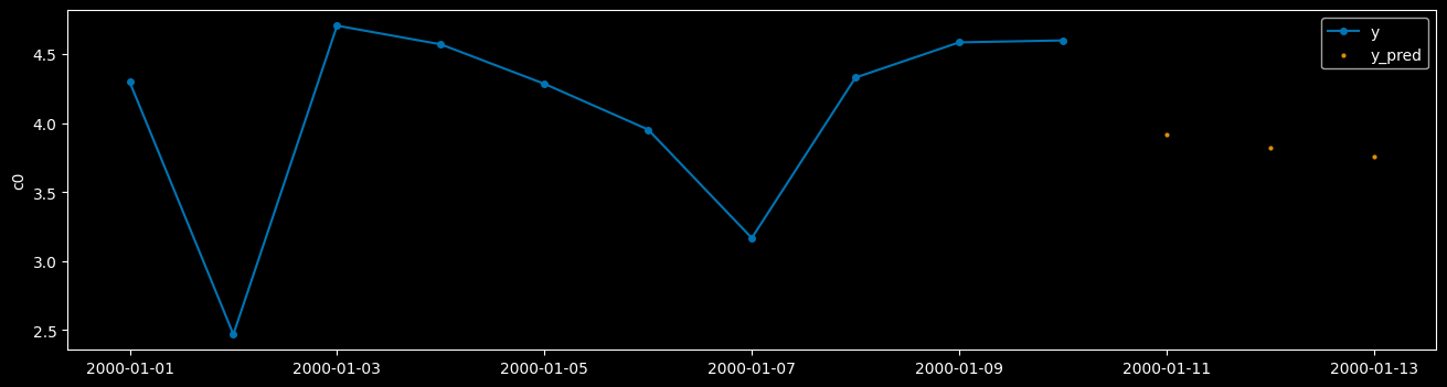
y_pred 具有与 y_test 相同的实例索引,即 h0_90 到 h0_99。
我们可以绘制一个时间序列来查看结果。由于我们使用的是随机数据并且只训练了几个 epoch,所以不能期望太高。
[39]:
from sktime.utils.plotting import plot_series

plot_series(
    y_test.loc[("h0_99")],
    y_pred.loc[("h0_99")],
    labels=["y", "y_pred"],
)
[39]:
(<Figure size 1600x400 with 1 Axes>, <Axes: ylabel='c0'>)
当我们使用外部数据进行预测时,我们需要将 X 和 y 都传递给 predict。
X 必须包含所有历史值和待预测的时间点,而 y 应仅包含历史值,但不包含待预测的时间点。
[40]:
from sklearn.model_selection import train_test_split

from sktime.utils._testing.hierarchical import _make_hierarchical

data = _make_hierarchical(
    hierarchy_levels=(100, 1), max_timepoints=10, min_timepoints=10, n_columns=2
)
data = data.droplevel(1)
x = data["c0"].to_frame()
y = data["c1"].to_frame()
X_train, X_test, y_train, y_test = train_test_split(
    x, y, test_size=0.1, train_size=0.9, shuffle=False
)
y_test = y_test.groupby(level=0).apply(lambda x: x.droplevel(0).iloc[:-3])
X_train 和 y_train 具有相同的日期索引,从 2000-01-01 到 2000-01-10。
然而 y_test 比 X_test 短。
X_test 的时间索引从 2000-01-01 到 2000-01-10,但 y_test 的时间索引仅从 2000-01-01 到 2000-01-07。
这是因为我们不知道 y_test 中从 2000-01-08 到 2000-01-10 的值,这些值将要被预测。
[41]:
y_test
[41]:
| c1 | ||
|---|---|---|
| h0 | time | |
| h0_90 | 2000-01-01 | 4.697726 |
| 2000-01-02 | 4.376547 | |
| 2000-01-03 | 4.419372 | |
| 2000-01-04 | 6.045622 | |
| 2000-01-05 | 4.986501 | |
| ... | ... | ... |
| h0_99 | 2000-01-03 | 3.633788 |
| 2000-01-04 | 5.149747 | |
| 2000-01-05 | 5.850804 | |
| 2000-01-06 | 3.724629 | |
| 2000-01-07 | 4.151905 |
70 行 × 1 列
y_test 比 X_test 短,因为 y_test 只包含历史值,而不包含待预测的时间点。
让我们初始化一个可以处理外部数据的全局预测器。
[42]:
from sktime.forecasting.pytorchforecasting import PytorchForecastingTFT
[43]:
model = PytorchForecastingTFT(
    trainer_params={
        "max_epochs": 5,  # for quick test
        "limit_train_batches": 10,  # for quick test
    },
    dataset_params={
        "max_encoder_length": 3,
    },
)
[44]:
model.fit(y=y_train, X=X_train, fh=fh)
GPU available: True (cuda), used: True
TPU available: False, using: 0 TPU cores
IPU available: False, using: 0 IPUs
HPU available: False, using: 0 HPUs
LOCAL_RANK: 0 - CUDA_VISIBLE_DEVICES: [0]

   | Name                               | Type                            | Params
----------------------------------------------------------------------------------------
0  | loss                               | QuantileLoss                    | 0
1  | logging_metrics                    | ModuleList                      | 0
2  | input_embeddings                   | MultiEmbedding                  | 0
3  | prescalers                         | ModuleDict                      | 32
4  | static_variable_selection          | VariableSelectionNetwork        | 0
5  | encoder_variable_selection         | VariableSelectionNetwork        | 1.2 K
6  | decoder_variable_selection         | VariableSelectionNetwork        | 528
7  | static_context_variable_selection  | GatedResidualNetwork            | 1.1 K
8  | static_context_initial_hidden_lstm | GatedResidualNetwork            | 1.1 K
9  | static_context_initial_cell_lstm   | GatedResidualNetwork            | 1.1 K
10 | static_context_enrichment          | GatedResidualNetwork            | 1.1 K
11 | lstm_encoder                       | LSTM                            | 2.2 K
12 | lstm_decoder                       | LSTM                            | 2.2 K
13 | post_lstm_gate_encoder             | GatedLinearUnit                 | 544
14 | post_lstm_add_norm_encoder         | AddNorm                         | 32
15 | static_enrichment                  | GatedResidualNetwork            | 1.4 K
16 | multihead_attn                     | InterpretableMultiHeadAttention | 676
17 | post_attn_gate_norm                | GateAddNorm                     | 576
18 | pos_wise_ff                        | GatedResidualNetwork            | 1.1 K
19 | pre_output_gate_norm               | GateAddNorm                     | 576
20 | output_layer                       | Linear                          | 119
----------------------------------------------------------------------------------------
15.5 K    Trainable params
0         Non-trainable params
15.5 K    Total params
0.062     Total estimated model params size (MB)
`Trainer.fit` stopped: `max_epochs=5` reached.
[44]:
PytorchForecastingTFT(dataset_params={'max_encoder_length': 3},
                      trainer_params={'limit_train_batches': 10,
                                      'max_epochs': 5})
请重新运行此单元格以显示 HTML 表示或信任 notebook。PytorchForecastingTFT(dataset_params={'max_encoder_length': 3},
trainer_params={'limit_train_batches': 10,
'max_epochs': 5})现在我们可以在 X_test 的基础上对 y_test 进行预测。
[45]:
y_pred = model.predict(fh=fh, X=X_test, y=y_test)
y_pred
GPU available: True (cuda), used: True
TPU available: False, using: 0 TPU cores
IPU available: False, using: 0 IPUs
HPU available: False, using: 0 HPUs
LOCAL_RANK: 0 - CUDA_VISIBLE_DEVICES: [0]
[45]:
| c1 | ||
|---|---|---|
| h0 | time | |
| h0_90 | 2000-01-08 | 5.293717 |
| 2000-01-09 | 5.416963 | |
| 2000-01-10 | 5.225151 | |
| h0_91 | 2000-01-08 | 5.403152 |
| 2000-01-09 | 5.357550 | |
| 2000-01-10 | 5.228848 | |
| h0_92 | 2000-01-08 | 4.887965 |
| 2000-01-09 | 5.358321 | |
| 2000-01-10 | 5.270049 | |
| h0_93 | 2000-01-08 | 4.839972 |
| 2000-01-09 | 5.394659 | |
| 2000-01-10 | 5.279878 | |
| h0_94 | 2000-01-08 | 5.108763 |
| 2000-01-09 | 5.272538 | |
| 2000-01-10 | 5.389787 | |
| h0_95 | 2000-01-08 | 5.334348 |
| 2000-01-09 | 5.442789 | |
| 2000-01-10 | 5.271264 | |
| h0_96 | 2000-01-08 | 5.372472 |
| 2000-01-09 | 5.166903 | |
| 2000-01-10 | 5.351241 | |
| h0_97 | 2000-01-08 | 5.397213 |
| 2000-01-09 | 5.419333 | |
| 2000-01-10 | 5.382102 | |
| h0_98 | 2000-01-08 | 4.978965 |
| 2000-01-09 | 5.106180 | |
| 2000-01-10 | 5.135403 | |
| h0_99 | 2000-01-08 | 5.401626 |
| 2000-01-09 | 5.305851 | |
| 2000-01-10 | 5.175489 |
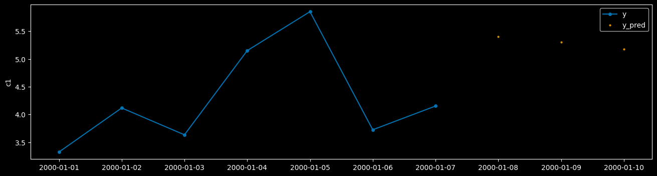
我们可以绘制一个时间序列来查看结果。由于我们使用的是随机数据并且只训练了几个 epoch,所以不能期望太高。
[46]:
plot_series(
    y_test.loc[("h0_99")],
    y_pred.loc[("h0_99")],
    labels=["y", "y_pred"],
)
[46]:
(<Figure size 1600x400 with 1 Axes>, <Axes: ylabel='c1'>)
构建您自己的层级或全局预测器#
入门
使用高级预测扩展模板
扩展模板 = 带有待办事项块的 Python“填写”模板,允许您实现自己的、与 sktime 兼容的预测算法。
使用 check_estimator 检查估计器
对于层级预测
确保为面板和层级数据选择受支持的 mtype
推荐:
y_inner_mtype = ["pd.DataFrame", "pd-multiindex", "pd_multiindex_hier"],X_inner_mtype也相同这确保在
_fit,_predict中看到的输入y,X是pd.DataFrame,具有 1、2、3 或更多行级别
如果存在高效的实现,您可以实现跨行的向量化
但是:自动化向量化已经遍历了行索引集,如果这就是“层级”的含义,请不要重复实现该功能
为了确保自动化向量化,请不要在
y_inner_mtype,X_inner_mtype中包含 Hierarchical 或 Panel mtypes
仔细思考您的估计器是预测器,还是可以分解为 Transformer
“执行 X 然后应用 sktime 中已有的预测器”是强烈暗示您实际上想要实现一个 Transformer
致谢#
notebook 创建:danbartl, fkiraly