![]()
使用 sktime 进行预测 - 附录:预测、监督回归以及混淆两者的陷阱#
本 notebook 提供了一些补充解释,阐述了 sktime 中实现的预测功能与 scikit-learn 及类似工具箱支持的常见监督预测任务之间的关系。
本 notebook 中讨论的关键点
预测与监督预测不同;
即使可以使用监督预测算法“解决”预测问题,这也是间接的,并且需要仔细组合;
从接口角度来看,这被正确地表述为“归约”,即在预测器中将监督预测器用作组件;
如果手动执行此操作,存在许多陷阱,例如过度乐观的性能评估、信息泄露或“预测过去”类型的错误。
[1]:
# general imports
import numpy as np
import pandas as pd
将预测错误地诊断为监督回归的陷阱#
一个常见的错误是将预测问题误认为监督回归——毕竟,两者都是预测数字,所以这肯定是一回事,对吧?
确实,两者都预测数字,但设置不同
在监督回归中,我们在横截面设置中从特征变量预测标签/目标变量。这是在标签/特征示例上训练之后。
在预测中,我们在时间/序列设置中根据过去的值预测未来的值,并且是同一变量。这是在过去数据上训练之后。
在常见的数据框表示中
在监督回归中,我们根据其他列预测某一列的条目。为此,我们主要利用从完整行示例中学到的这些列之间的统计关系。所有行都被认为是可交换的。
在预测中,我们预测新的行,假设行中存在时间顺序。为此,我们主要利用从观察到的行序列示例中学到的前一行和后一行之间的统计关系。这些行不可交换,而是按时间顺序排列。
陷阱 1:性能评估中的过度乐观,对“失效”预测器的虚假信心#
混淆这两项任务可能导致信息泄露和过度乐观的性能评估。这是因为在监督回归中,行的顺序无关紧要,并且训练/测试分割通常是均匀进行的。而在预测中,顺序很重要,无论是在训练还是在评估中。
尽管这看似微妙,但可能产生重大的实际后果——因为这可能导致错误地认为一个“失效”的方法是有效的,从而在实际部署中对健康、财产和其他资产造成损害。
以下示例展示了将回归评估工作流程误用于预测时,“有问题”的性能估计。
[2]:
from sklearn.model_selection import train_test_split

from sktime.datasets import load_airline
from sktime.split import temporal_train_test_split
from sktime.utils.plotting import plot_series
[3]:
y = load_airline()
[4]:
y_train, y_test = train_test_split(y)
plot_series(y_train.sort_index(), y_test.sort_index(), labels=["y_train", "y_test"]);
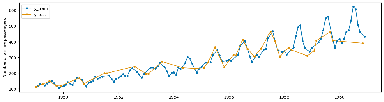
这会导致泄露
您用于训练机器学习算法的数据恰好包含您试图预测的信息。
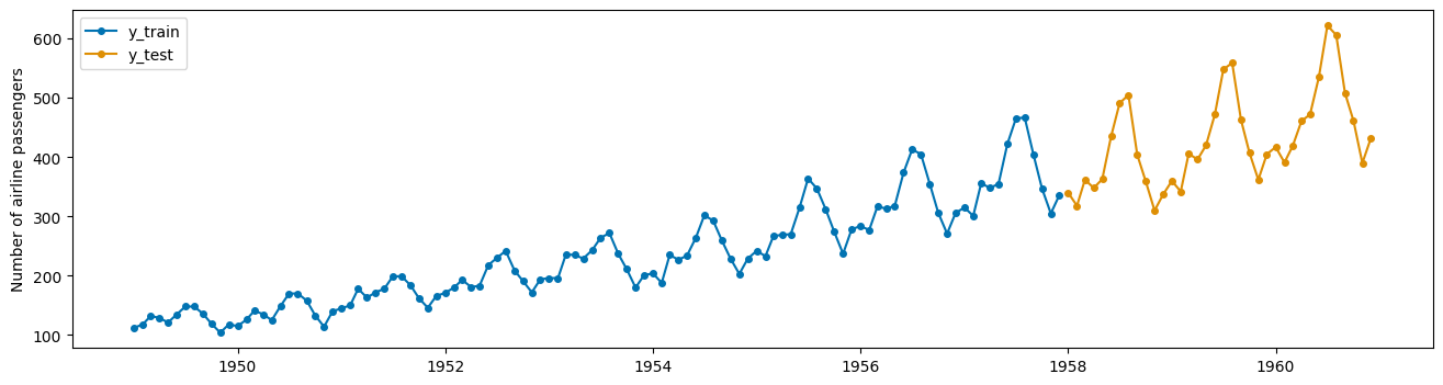
但是 train_test_split(y, shuffle=False) 是有效的,这与 sktime 中 temporal_train_test_split(y) 的作用相同。
[5]:
y_train, y_test = temporal_train_test_split(y)
plot_series(y_train, y_test, labels=["y_train", "y_test"]);
陷阱 2:晦涩的数据操作,脆弱的套路代码以应用回归器#
将数据转换为用于预测的形式(通过滞后处理,例如在自回归归约策略中)后应用监督回归器是一种常见做法。
从一开始就出现两个重要的陷阱
需要编写大量套路代码来转换数据以使其适合拟合——这极易出错
这里存在许多隐式超参数,例如窗口大小和滞后大小。如果不谨慎处理,这些参数不会明确或在实验中被跟踪,这可能导致“p 值操纵”。
下面是展示此问题的套路代码示例。该代码紧密模仿了 M4 竞赛中使用的 R 代码。
[6]:
# suppose we want to predict 3 years ahead
fh = np.arange(1, 37)
[7]:
# slightly modified code from the M4 competition


def split_into_train_test(data, in_num, fh):
    """Split the series into train and test sets.

    Each step takes multiple points as inputs
    :param data: an individual TS
    :param fh: number of out of sample points
    :param in_num: number of input points for the forecast
    :return:
    """
    train, test = data[:-fh], data[-(fh + in_num) :]
    x_train, y_train = train[:-1], np.roll(train, -in_num)[:-in_num]
    x_test, y_test = test[:-1], np.roll(test, -in_num)[:-in_num]
    #     x_test, y_test = train[-in_num:], np.roll(test, -in_num)[:-in_num]

    # reshape input to be [samples, time steps, features]
    # (N-NF samples, 1 time step, 1 feature)
    x_train = np.reshape(x_train, (-1, 1))
    x_test = np.reshape(x_test, (-1, 1))
    temp_test = np.roll(x_test, -1)
    temp_train = np.roll(x_train, -1)
    for _ in range(1, in_num):
        x_train = np.concatenate((x_train[:-1], temp_train[:-1]), 1)
        x_test = np.concatenate((x_test[:-1], temp_test[:-1]), 1)
        temp_test = np.roll(temp_test, -1)[:-1]
        temp_train = np.roll(temp_train, -1)[:-1]

    return x_train, y_train, x_test, y_test
[8]:
# here we split the time index, rather than the actual values,
# to show how we split the windows
feature_window, target_window, _, _ = split_into_train_test(
    np.arange(len(y)), 10, len(fh)
)
为了更好地理解之前的数据转换,我们可以看看如何将训练序列分割成窗口。这里我们展示了以整数索引表示的生成的窗口。
[9]:
feature_window[:5, :]
[9]:
array([[ 0,  1,  2,  3,  4,  5,  6,  7,  8,  9],
       [ 1,  2,  3,  4,  5,  6,  7,  8,  9, 10],
       [ 2,  3,  4,  5,  6,  7,  8,  9, 10, 11],
       [ 3,  4,  5,  6,  7,  8,  9, 10, 11, 12],
       [ 4,  5,  6,  7,  8,  9, 10, 11, 12, 13]])
[10]:
target_window[:5]
[10]:
array([10, 11, 12, 13, 14])
[11]:
# now we can split the actual values of the time series
x_train, y_train, x_test, y_test = split_into_train_test(y.values, 10, len(fh))
print(x_train.shape, y_train.shape)
(98, 10) (98,)
[12]:
from sklearn.ensemble import RandomForestRegressor

model = RandomForestRegressor()
model.fit(x_train, y_train)
[12]:
RandomForestRegressor()在 Jupyter 环境中,请重新运行此单元格以显示 HTML 表示或信任此 notebook。
在 GitHub 上,HTML 表示无法渲染,请尝试使用 nbviewer.org 加载此页面。
RandomForestRegressor()
重申这里的潜在陷阱
手动操作需要编写大量手写代码,这通常容易出错、不模块化且不可调。
这些步骤涉及许多隐式超参数
您将时间序列分割成窗口的方式(例如窗口长度);
您生成预测的方式(递归策略、直接策略、其他混合策略)。
陷阱 3:给定一个已拟合的回归算法,如何生成预测?#
下一个重要陷阱出现在最后
如果沿着监督回归器的“手动路线”进行预测,监督回归器的输出必须转换回预测结果。这很容易被遗忘,并导致预测和评估中的错误(参见陷阱 1)——特别是如果无法清晰地跟踪在何时知道哪些数据,或如何反转拟合时进行的转换。
一个新手用户可能会这样操作
[13]:
print(x_test.shape, y_test.shape)

# add back time index to y_test
y_test = pd.Series(y_test, index=y.index[-len(fh) :])
(36, 10) (36,)
[14]:
y_pred = model.predict(x_test)
[15]:
from sktime.performance_metrics.forecasting import mean_absolute_percentage_error

mean_absolute_percentage_error(
    y_test, pd.Series(y_pred, index=y_test.index), symmetric=False
)
[15]:
0.10892546588134275
如此简单,如此错误……但问题出在哪里?这有点微妙,不容易发现。
我们实际上并没有进行最多 36 步远的多元预测。相反,我们进行了 36 次单步预测,始终使用最新的数据。但这解决的是一个不同的学习任务!
为了解决这个问题,我们可以编写一些代码来像 M4 竞赛那样递归地执行此操作
[16]:
# slightly modified code from the M4 study
predictions = []
last_window = x_train[-1, :].reshape(1, -1)  # make it into 2d array

last_prediction = model.predict(last_window)[0]  # take value from array

for i in range(len(fh)):
    # append prediction
    predictions.append(last_prediction)

    # update last window using previously predicted value
    last_window[0] = np.roll(last_window[0], -1)
    last_window[0, (len(last_window[0]) - 1)] = last_prediction

    # predict next step ahead
    last_prediction = model.predict(last_window)[0]

y_pred_rec = pd.Series(predictions, index=y_test.index)
[17]:
from sktime.performance_metrics.forecasting import mean_absolute_percentage_error

mean_absolute_percentage_error(
    y_test, pd.Series(y_pred_rec, index=y_test.index), symmetric=False
)
[17]:
0.19738808156953527
总结这里的潜在陷阱
获取回归器预测并将其转换回预测结果并非易事且容易出错
需要编写一些套路代码,这就像陷阱 2 一样会引入潜在问题;
从一开始就必须编写这些套路代码并不那么明显,这会产生一个微妙的故障点。
sktime 如何帮助避免上述陷阱?#
sktime 通过以下方式减轻了上述陷阱
其统一的预测器接口——任何生成预测的策略都是一个预测器。通过统一接口,预测器直接与适用于预测器的部署和评估工作流程兼容;
其声明式规范接口最大限度地减少了套路代码——它被最小化到仅需告诉
sktime您想构建哪个预测器。
尽管如此,sktime 旨在保持灵活性,并尽量避免强制用户采用特定的方法选择。
[18]:
from sklearn.neighbors import KNeighborsRegressor

from sktime.forecasting.compose import make_reduction
[19]:
# declarative forecaster specification - just two lines!
regressor = KNeighborsRegressor(n_neighbors=1)
forecaster = make_reduction(regressor, window_length=15, strategy="recursive")
[20]:
forecaster.fit(y_train)
y_pred = forecaster.predict(fh)
……就是这样!
注意,这里没有 x_train 或其他套路代码产物,因为滞后特征的构建和其他套路代码由预测器内部处理。
有关 sktime 组合接口的更多详细信息,请参阅主要预测教程的第 3 节。