sktime 中的 Transformer#

本 notebook 概览#

为什么使用 transformer？sktime 中的 transformer
- transformer = 模块化数据处理步骤
- 简单管道示例和 transformer 解释

transformer 功能概览
- transformer 类型 - 输入类型、输出类型
- 广播/向量化到面板、层级、多元
- 使用 all_estimators 搜索 transformer

[1]:

import warnings

warnings.filterwarnings("ignore")

目录#

3. sktime 中的 Transformer
- 3.1 为何使用 transformer？
- 3.2 Transformer - 接口和功能
  - 3.2.1 什么是 transformer？
  - 3.2.2 不同类型的 transformer
  - 3.2.3 transformer 的广播或向量化
  - 3.2.4 作为管道组件的 transformer
- 3.3 组合 transformer，特征工程
- 3.4 技术细节 - transformer 类型和签名
- 3.5 扩展指南
- 3.6 总结

3.1 为何使用 transformer？#

或者：为什么 sktime 中的 transformer 将改善你的生活！

(免责声明：与深度学习中的 transformer 不是同一产品)

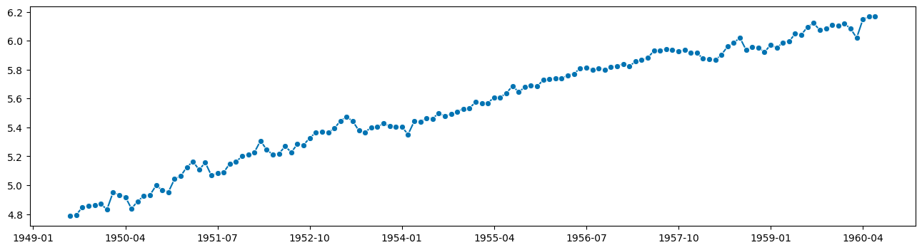
假设我们要预测这个著名数据集（特定范围内的年度航空旅客）

[2]:

from sktime.datasets import load_airline
from sktime.utils.plotting import plot_series

y = load_airline()
plot_series(y)

[2]:

(<Figure size 1600x400 with 1 Axes>,
 <AxesSubplot: ylabel='Number of airline passengers'>)

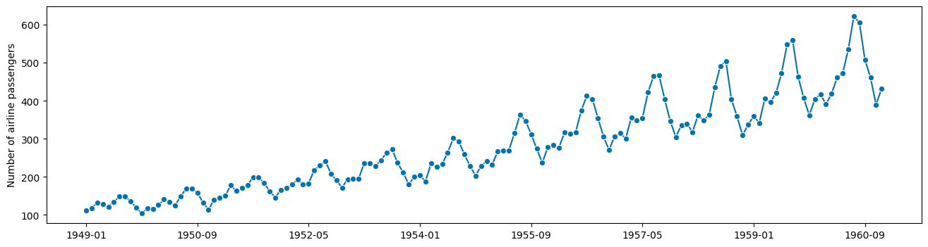
../_images/examples_03_transformers_8_1.png

观察结果

存在季节性周期性，周期为 12 个月
季节性周期性看起来与趋势是乘法关系（非加法关系）

想法：预测可能更容易

去除季节性后
在对数值尺度上（乘法变为加法）

朴素方法 - 请勿在家尝试！#

也许手动一步步来是个好主意？

[3]:

import numpy as np

# compute the logarithm
logy = np.log(y)

plot_series(logy)

[3]:

(<Figure size 1600x400 with 1 Axes>,
 <AxesSubplot: ylabel='Number of airline passengers'>)

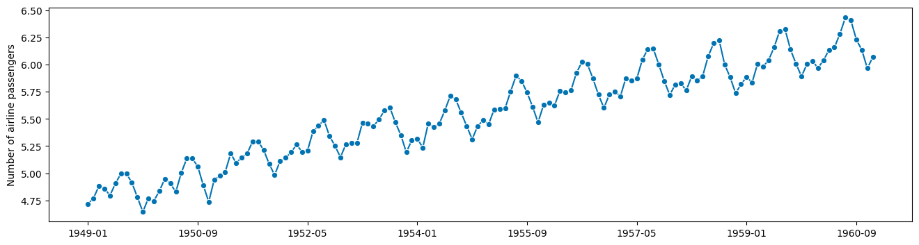
../_images/examples_03_transformers_12_1.png

现在看起来是加法关系了！

好的，接下来是什么 - 去除季节性

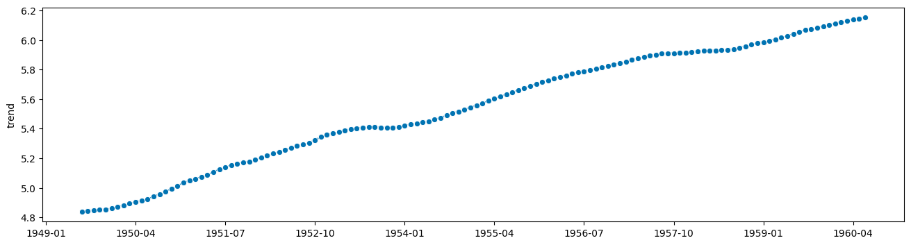
[4]:

from statsmodels.tsa.seasonal import seasonal_decompose

# apply this to y
# wait no, to logy

seasonal_result = seasonal_decompose(logy, period=12)

trend = seasonal_result.trend
resid = seasonal_result.resid
seasonal = seasonal_result.seasonal

[5]:

plot_series(trend)

[5]:

(<Figure size 1600x400 with 1 Axes>, <AxesSubplot: ylabel='trend'>)

../_images/examples_03_transformers_15_1.png

[6]:

plot_series(seasonal, resid, labels=["seasonal component", "residual component"])

[6]:

(<Figure size 1600x400 with 1 Axes>, <AxesSubplot: ylabel='seasonal'>)

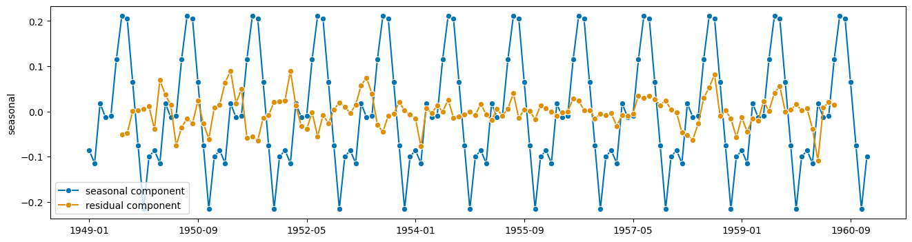
../_images/examples_03_transformers_16_1.png

好的，现在进行预测！

… 预测什么？？

啊，对了，残差加趋势，因为季节性只是重复自身

[7]:

# forecast this:
plot_series(trend + resid)

[7]:

(<Figure size 1600x400 with 1 Axes>, <AxesSubplot: >)

../_images/examples_03_transformers_18_1.png

[8]:

# this has nans??
trend

[8]:

1949-01   NaN
1949-02   NaN
1949-03   NaN
1949-04   NaN
1949-05   NaN
           ..
1960-08   NaN
1960-09   NaN
1960-10   NaN
1960-11   NaN
1960-12   NaN
Freq: M, Name: trend, Length: 144, dtype: float64

[9]:

# ok, forecast this instead then:
y_to_forecast = logy - seasonal

# phew, no nans!
y_to_forecast

[9]:

1949-01    4.804314
1949-02    4.885097
1949-03    4.864689
1949-04    4.872858
1949-05    4.804757
             ...
1960-08    6.202368
1960-09    6.165645
1960-10    6.208669
1960-11    6.181992
1960-12    6.168741
Freq: M, Length: 144, dtype: float64

[10]:

from sktime.forecasting.trend import PolynomialTrendForecaster

f = PolynomialTrendForecaster(degree=2)
f.fit(y_to_forecast, fh=list(range(1, 13)))
y_fcst = f.predict()

plot_series(y_to_forecast, y_fcst)

[10]:

(<Figure size 1600x400 with 1 Axes>, <AxesSubplot: >)

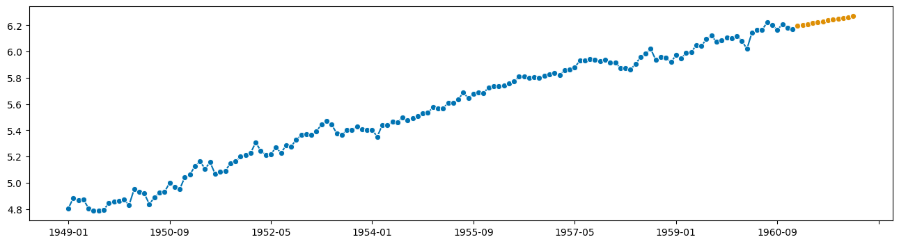
../_images/examples_03_transformers_21_1.png

看起来合理！

现在要把这变成原始 y 的预测…

加上季节性
反转对数变换

[11]:

y_fcst

[11]:

1961-01    6.195931
1961-02    6.202857
1961-03    6.209740
1961-04    6.216580
1961-05    6.223378
1961-06    6.230132
1961-07    6.236843
1961-08    6.243512
1961-09    6.250137
1961-10    6.256719
1961-11    6.263259
1961-12    6.269755
Freq: M, dtype: float64

[12]:

y_fcst_orig = y_fcst + seasonal[0:12]
y_fcst_orig_orig = np.exp(y_fcst_orig)

y_fcst_orig_orig

[12]:

1949-01   NaN
1949-02   NaN
1949-03   NaN
1949-04   NaN
1949-05   NaN
1949-06   NaN
1949-07   NaN
1949-08   NaN
1949-09   NaN
1949-10   NaN
1949-11   NaN
1949-12   NaN
1961-01   NaN
1961-02   NaN
1961-03   NaN
1961-04   NaN
1961-05   NaN
1961-06   NaN
1961-07   NaN
1961-08   NaN
1961-09   NaN
1961-10   NaN
1961-11   NaN
1961-12   NaN
Freq: M, dtype: float64

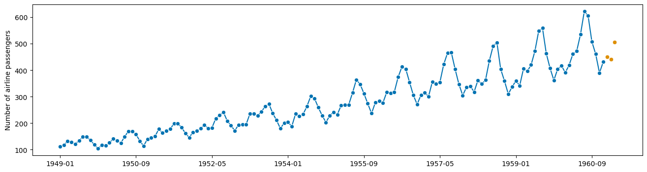
好的，这没起作用。是不是 pandas 索引出了什么问题？？

[13]:

y_fcst_orig = y_fcst + seasonal[0:12].values
y_fcst_orig_orig = np.exp(y_fcst_orig)

plot_series(y, y_fcst_orig_orig)

[13]:

(<Figure size 1600x400 with 1 Axes>,
 <AxesSubplot: ylabel='Number of airline passengers'>)

../_images/examples_03_transformers_26_1.png

好的，完成了！只花了我们 10 年时间。

也许有更好的方法？

稍微不那么朴素的方法 - (糟糕地) 使用 `sktime` 中的 transformer#

好的，肯定有一种方法让我不必摆弄每个步骤差异巨大的接口。

解决方案：使用 transformer！

每个步骤使用相同的接口！

[14]:

from sktime.forecasting.trend import PolynomialTrendForecaster
from sktime.transformations.series.boxcox import LogTransformer
from sktime.transformations.series.detrend import Deseasonalizer

y = load_airline()

t_log = LogTransformer()
ylog = t_log.fit_transform(y)

t_deseason = Deseasonalizer(sp=12)
y_deseason = t_deseason.fit_transform(ylog)

f = PolynomialTrendForecaster(degree=2)
f.fit(y_deseason, fh=list(range(1, 13)))
y_fcst = f.predict()

嗯，但现在我们需要反转这些变换…

幸运的是，transformer 具有逆变换功能，这是一个标准接口点

[15]:

y_fcst_orig = t_deseason.inverse_transform(y_fcst)
# the deseasonalizer remembered the seasonality component! nice!

y_fcst_orig_orig = t_log.inverse_transform(y_fcst_orig)

plot_series(y, y_fcst_orig_orig)

[15]:

(<Figure size 1600x400 with 1 Axes>,
 <AxesSubplot: ylabel='Number of airline passengers'>)

../_images/examples_03_transformers_31_1.png

专家方法 - 使用 sktime 中的 transformer 构建管道！#

包含炫耀资本。

[16]:

from sktime.forecasting.trend import PolynomialTrendForecaster
from sktime.transformations.series.boxcox import LogTransformer
from sktime.transformations.series.detrend import Deseasonalizer

y = load_airline()

f = LogTransformer() * Deseasonalizer(sp=12) * PolynomialTrendForecaster(degree=2)

f.fit(y, fh=list(range(1, 13)))
y_fcst = f.predict()

plot_series(y, y_fcst)

[16]:

(<Figure size 1600x400 with 1 Axes>,
 <AxesSubplot: ylabel='Number of airline passengers'>)

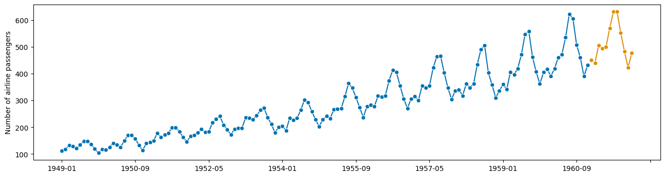
../_images/examples_03_transformers_33_1.png

这里发生了什么？

“链式”运算符 * 创建了一个“预测管道”

与所有其他预测器具有相同的接口！无需额外的数据处理！

Transformer 作为标准化组件“插槽”其中。

[17]:

[17]:

TransformedTargetForecaster(steps=[LogTransformer(), Deseasonalizer(sp=12),
                                   PolynomialTrendForecaster(degree=2)])

在 Jupyter 环境中，请重新运行此单元格以显示 HTML 表示或信任 notebook。
在 GitHub 上，HTML 表示无法渲染，请尝试使用 nbviewer.org 加载此页面。

让我们更详细地看一下

sktime transformer 接口
sktime 管道构建

3.2 Transformer - 接口和功能#

transformer 接口
transformer 类型
按类型搜索 transformer
广播/向量化到面板和层级数据
transformer 和管道

3.2.1 什么是 transformer？#

Transformer = 机器学习中常用的模块化数据处理步骤

（“transformer” 的用法与 scikit-learn 中的一致）

Transformer 是以下类型的评估器：

通过 fit(data) 对一批数据进行拟合，改变其状态
通过 transform(X) 应用于另一批数据，生成转换后的数据
可能具有 inverse_transform(X) 方法

在 sktime 中，fit 和 transform 的输入 X 通常是时间序列或面板（时间序列集合）。

sktime 时间序列 transformer 的基本用法如下：

[18]:

# 1. prepare the data
from sktime.utils._testing.series import _make_series

X = _make_series()
X_train = X[:7]
X_test = X[7:12]
# X_train and X_test are both pandas.Series

X_train, X_test

[18]:

(2000-01-01    4.708975
 2000-01-02    1.803052
 2000-01-03    2.403074
 2000-01-04    3.076577
 2000-01-05    2.902616
 2000-01-06    3.831219
 2000-01-07    2.121627
 Freq: D, dtype: float64,
 2000-01-08    4.858755
 2000-01-09    3.460329
 2000-01-10    2.280978
 2000-01-11    1.930733
 2000-01-12    4.604839
 Freq: D, dtype: float64)

[19]:

# 2. construct the transformer
from sktime.transformations.series.boxcox import BoxCoxTransformer

# trafo is an sktime estimator inheriting from BaseTransformer
# Box-Cox transform with lambda parameter fitted via mle
trafo = BoxCoxTransformer(method="mle")

[20]:

# 3. fit the transformer to training data
trafo.fit(X_train)

# 4. apply the transformer to transform test data
# Box-Cox transform with lambda fitted on X_train
X_transformed = trafo.transform(X_test)

X_transformed

[20]:

2000-01-08    1.242107
2000-01-09    1.025417
2000-01-10    0.725243
2000-01-11    0.593567
2000-01-12    1.209380
Freq: D, dtype: float64

如果训练集和测试集相同，可以使用 fit_transform 更简洁（有时也更高效）地执行步骤 3 和 4

[21]:

# 3+4. apply the transformer to fit and transform on the same data, X
X_transformed = trafo.fit_transform(X)

3.2.2 不同类型的 transformer#

sktime 根据 fit 和 transform 的输入类型以及 transform 的输出类型，区分了不同类型的 transformer。

Transformer 的区别在于：

在 fit 或 transform 中使用额外的 y 参数
fit 和 transform 的输入是单个时间序列、时间序列集合还是标量值（数据框行）
transform 的输出是单个时间序列、时间序列集合还是标量值（数据框行）
fit 和 transform 的输入是一个对象还是两个。输入是两个对象且输出是标量值表示该 transformer 是距离或核函数。

更多详细信息请参见词汇表（第 2.3 节）。

为了说明差异，我们比较两个输出不同的 transformer

Box-Cox transformer BoxCoxTrannsformer，它将时间序列转换为时间序列
摘要 transformer SummaryTransformer，它将时间序列转换为标量值，例如均值

[22]:

# constructing the transformer
from sktime.transformations.series.boxcox import BoxCoxTransformer
from sktime.transformations.series.summarize import SummaryTransformer
from sktime.utils._testing.series import _make_series

# getting some data
# this is one pandas.Series
X = _make_series(n_timepoints=10)

# constructing the transformers
boxcox_trafo = BoxCoxTransformer(method="mle")
summary_trafo = SummaryTransformer()

[23]:

# this produces a pandas Series
boxcox_trafo.fit_transform(X)

[23]:

2000-01-01    3.217236
2000-01-02    6.125564
2000-01-03    5.264381
2000-01-04    3.811121
2000-01-05    1.966839
2000-01-06    2.621609
2000-01-07    3.851400
2000-01-08    3.199416
2000-01-09    0.000000
2000-01-10    6.629380
Freq: D, dtype: float64

[24]:

# this produces a pandas.DataFrame row
summary_trafo.fit_transform(X)

[24]:

	均值	标准差	最小值	最大值	0.1	0.25	0.5	0.75	0.9
0	3.368131	1.128705	1.0	4.881081	2.339681	2.963718	3.376426	4.0816	4.67824

对于时间序列 transformer，元数据标签描述了 transform 的预期输出

[25]:

boxcox_trafo.get_tag("scitype:transform-output")

[25]:

'Series'

[26]:

summary_trafo.get_tag("scitype:transform-output")

[26]:

'Primitives'

要查找 transformer，使用 all_estimators 并按标签过滤

"scitype:transform-output" - 输出科学类型。时间序列为 Series，原始特征（浮点数、类别）为 Primitives，时间序列集合为 Panel。
"scitype:transform-input" - 输入科学类型。时间序列为 Series。
"scitype:instancewise" - 如果为 True，则对每个时间序列进行向量化操作。如果为 False，则非平凡地使用多个时间序列。

示例：查找所有输出时间序列的 transformer

[27]:

from sktime.registry import all_estimators

# now subset to transformers that extract scalar features
all_estimators(
    "transformer",
    as_dataframe=True,
    filter_tags={"scitype:transform-output": "Series"},
)

Importing plotly failed. Interactive plots will not work.

[27]:

	名称	评估器
0	Aggregator	<class 'sktime.transformations.hierarchical.ag...'>
1	AutoCorrelationTransformer	<class 'sktime.transformations.series.acf.Auto...'>
2	BoxCoxTransformer	<class 'sktime.transformations.series.boxcox.B...'>
3	ClaSPTransformer	<class 'sktime.transformations.series.clasp.Cl...'>
4	ClearSky	<class 'sktime.transformations.series.clear_sk...'>
...	...	...
69	TransformerPipeline	<class 'sktime.transformations.compose.Transfo...'>
70	TruncationTransformer	<class 'sktime.transformations.panel.truncatio...'>
71	WhiteNoiseAugmenter	<class 'sktime.transformations.series.augmente...'>
72	WindowSummarizer	<class 'sktime.transformations.series.summariz...'>
73	YtoX	<class 'sktime.transformations.compose.YtoX'>

74 行 × 2 列

关于 transformer 类型和标签的更完整概览在 sktime transformer 教程中提供。

3.2.3 transformer 的广播或向量化#

sktime 中的 transformer 可能原本是单变量的，或仅应用于单个时间序列。

即使如此，它们也会在适用时跨变量和时间序列实例进行广播（在 numpy 术语中也称为向量化）。

这确保了所有 sktime transformer 都可以应用于多元和多实例（面板、层级）时间序列数据。

示例 1：时间序列到时间序列 transformer 的广播/向量化

前面的章节中的 BoxCoxTransformer 应用于单变量时间序列的单个实例。当遇到多个实例或变量时，它会同时在这两者之间进行广播

[28]:

from sktime.transformations.series.boxcox import BoxCoxTransformer
from sktime.utils._testing.hierarchical import _make_hierarchical

# hierarchical data with 2 variables and 2 levels
X = _make_hierarchical(n_columns=2)

X

[28]:

			c0	c1
h0	h1	时间
h0_0	h1_0	2000-01-01	3.068024	3.177475
		2000-01-02	2.917533	3.615065
		2000-01-03	3.654595	3.327944
		2000-01-04	2.848652	4.694433
		2000-01-05	3.458690	3.349914
...	...	...	...	...
h0_1	h1_3	2000-01-08	4.056444	3.726508
		2000-01-09	2.462253	3.938115
		2000-01-10	2.689640	1.000000
		2000-01-11	1.233706	3.999155
		2000-01-12	3.101318	3.632666

96 行 × 2 列

[29]:

# constructing the transformers
boxcox_trafo = BoxCoxTransformer(method="mle")

# applying to X results in hierarchical data
boxcox_trafo.fit_transform(X)

[29]:

			c0	c1
h0	h1	时间
h0_0	h1_0	2000-01-01	0.307301	3.456645
		2000-01-02	0.305723	4.416187
		2000-01-03	0.311191	3.777609
		2000-01-04	0.304881	7.108861
		2000-01-05	0.310189	3.825267
...	...	...	...	...
h0_1	h1_3	2000-01-08	1.884165	9.828613
		2000-01-09	1.087370	11.311330
		2000-01-10	1.216886	0.000000
		2000-01-11	0.219210	11.761224
		2000-01-12	1.435712	9.208733

96 行 × 2 列

向量化 transformer 的拟合模型组件可以在 transformers_ 属性中找到，或通过通用的 get_fitted_params 接口访问

[30]:

boxcox_trafo.transformers_
# this is a pandas.DataFrame that contains the fitted transformers
# one per time series instance and variable

[30]:

		c0	c1
h0	h1
h0_0	h1_0	BoxCoxTransformer()	BoxCoxTransformer()
	h1_1	BoxCoxTransformer()	BoxCoxTransformer()
	h1_2	BoxCoxTransformer()	BoxCoxTransformer()
	h1_3	BoxCoxTransformer()	BoxCoxTransformer()
h0_1	h1_0	BoxCoxTransformer()	BoxCoxTransformer()
	h1_1	BoxCoxTransformer()	BoxCoxTransformer()
	h1_2	BoxCoxTransformer()	BoxCoxTransformer()
	h1_3	BoxCoxTransformer()	BoxCoxTransformer()

[31]:

boxcox_trafo.get_fitted_params()
# this returns a dictionary
# the transformers DataFrame is available at the key "transformers"
# individual transformers are available at dataframe-like keys
# it also contains all fitted lambdas as keyed parameters

[31]:

{'transformers':                             c0                   c1
 h0   h1
 h0_0 h1_0  BoxCoxTransformer()  BoxCoxTransformer()
      h1_1  BoxCoxTransformer()  BoxCoxTransformer()
      h1_2  BoxCoxTransformer()  BoxCoxTransformer()
      h1_3  BoxCoxTransformer()  BoxCoxTransformer()
 h0_1 h1_0  BoxCoxTransformer()  BoxCoxTransformer()
      h1_1  BoxCoxTransformer()  BoxCoxTransformer()
      h1_2  BoxCoxTransformer()  BoxCoxTransformer()
      h1_3  BoxCoxTransformer()  BoxCoxTransformer(),
 "transformers.loc[('h0_0', 'h1_0'),c0]": BoxCoxTransformer(),
 "transformers.loc[('h0_0', 'h1_0'),c0]__lambda": -3.1599525634239187,
 "transformers.loc[('h0_0', 'h1_1'),c1]": BoxCoxTransformer(),
 "transformers.loc[('h0_0', 'h1_1'),c1]__lambda": 0.37511296223989965}

示例 2：时间序列到标量特征 transformer 的广播/向量化

SummaryTransformer 的行为类似。多个时间序列实例被转换为结果数据框的不同列。

[32]:

from sktime.transformations.series.summarize import SummaryTransformer

summary_trafo = SummaryTransformer()

# this produces a pandas DataFrame with more rows and columns
# rows correspond to different instances in X
# columns are multiplied and names prefixed by [variablename]__
# there is one column per variable and transformed feature
summary_trafo.fit_transform(X)

[32]:

		c0__mean	c0__std	c0__min	c0__max	c0__0.1	c0__0.25	c0__0.5	c0__0.75	c0__0.9	c1__mean	c1__std	c1__min	c1__max	c1__0.1	c1__0.25	c1__0.5	c1__0.75	c1__0.9
h0	h1
h0_0	h1_0	3.202174	0.732349	2.498101	5.283440	2.709206	2.834797	2.975883	3.348140	3.635005	3.360042	0.744295	1.910203	4.694433	2.278782	3.194950	3.377147	3.722876	3.981182
	h1_1	2.594633	0.850142	1.000000	4.040674	1.618444	1.988190	2.742309	3.084133	3.349082	3.637274	1.006419	2.376048	5.112509	2.402845	2.703573	3.644124	4.535796	4.873311
	h1_2	3.649374	1.181054	1.422356	5.359634	2.249409	2.881057	3.813969	4.319322	5.021987	2.945555	1.245355	1.684464	6.469536	1.795508	2.324243	2.757053	3.159779	3.547420
	h1_3	2.865339	0.745604	1.654998	4.718420	2.313490	2.477173	2.839630	3.137472	3.372838	3.394633	0.971250	1.866518	5.236633	2.506371	2.653524	3.259750	4.192159	4.419325
h0_1	h1_0	2.946692	1.025167	1.085568	5.159135	1.933525	2.375844	2.952310	3.412478	3.687086	3.203431	0.970914	1.554428	4.546142	1.756260	2.405147	3.544128	3.954901	4.046171
	h1_1	3.274710	0.883594	1.930773	4.771649	1.988411	2.710401	3.434244	3.799033	4.167242	3.116279	0.604060	2.235531	4.167924	2.426392	2.655720	3.079178	3.660901	3.762036
	h1_2	3.397527	0.630344	2.277090	4.571272	2.791987	2.965040	3.457581	3.783002	4.031893	3.297039	0.938834	1.826276	4.919249	2.292343	2.646870	3.139703	3.975298	4.365553
	h1_3	3.356722	1.326547	1.233706	5.505544	2.467667	2.567089	2.884737	4.308726	5.273261	3.232578	1.003957	1.000000	4.234051	2.113028	2.568151	3.659943	3.953375	4.022143

3.2.4 作为管道组件的 transformer#

sktime 中的 transformer 可以与任何其他 sktime 评估器类型构建管道，包括预测器、分类器和其他 transformer。

管道 = 同类型评估器，与专用类具有相同的接口

管道构建操作：make_pipeline 或通过 * dunder 方法

管道化 pipe = trafo * est 生成与 est 相同类型的 pipe。

在 pipe.fit 中，首先执行 trafo.fit_transform，然后在结果上执行 est.fit。

在 pipe.predict 中，首先执行 trafo.transform，然后执行 est.predict。

（管道传递的参数因类型而异，可以在管道类的文档字符串或专门的教程中查找）

我们已经在上面看到过这个示例

[33]:

from sktime.forecasting.trend import PolynomialTrendForecaster
from sktime.transformations.series.boxcox import LogTransformer
from sktime.transformations.series.detrend import Deseasonalizer

y = load_airline()

pipe = LogTransformer() * Deseasonalizer(sp=12) * PolynomialTrendForecaster(degree=2)

pipe

[33]:

TransformedTargetForecaster(steps=[LogTransformer(), Deseasonalizer(sp=12),
                                   PolynomialTrendForecaster(degree=2)])

在 Jupyter 环境中，请重新运行此单元格以显示 HTML 表示或信任 notebook。
在 GitHub 上，HTML 表示无法渲染，请尝试使用 nbviewer.org 加载此页面。

[34]:

# this is a forecaster with the same interface as Polynomial Trend Forecaster
pipe.fit(y, fh=[1, 2, 3])
y_pred = pipe.predict()

plot_series(y, y_pred)

[34]:

(<Figure size 1600x400 with 1 Axes>,
 <AxesSubplot: ylabel='Number of airline passengers'>)

../_images/examples_03_transformers_69_1.png

与分类器或其他评估器类型的工作方式相同！

[35]:

from sktime.classification.distance_based import KNeighborsTimeSeriesClassifier
from sktime.transformations.series.exponent import ExponentTransformer

pipe = ExponentTransformer() * KNeighborsTimeSeriesClassifier()

# this constructs a ClassifierPipeline, which is also a classifier
pipe

[35]:

ClassifierPipeline(classifier=KNeighborsTimeSeriesClassifier(),
                   transformers=[ExponentTransformer()])

在 Jupyter 环境中，请重新运行此单元格以显示 HTML 表示或信任 notebook。
在 GitHub 上，HTML 表示无法渲染，请尝试使用 nbviewer.org 加载此页面。

[36]:

from sktime.datasets import load_unit_test

X_train, y_train = load_unit_test(split="TRAIN")
X_test, _ = load_unit_test(split="TEST")

# this is a forecaster with the same interface as knn-classifier
# first applies exponent transform, then knn-classifier
pipe.fit(X_train, y_train)

[36]:

ClassifierPipeline(classifier=KNeighborsTimeSeriesClassifier(),
                   transformers=[ExponentTransformer()])

在 Jupyter 环境中，请重新运行此单元格以显示 HTML 表示或信任 notebook。
在 GitHub 上，HTML 表示无法渲染，请尝试使用 nbviewer.org 加载此页面。

3.3 组合 transformer，特征工程#

transformer 是天然的管道组件

数据处理步骤
特征工程步骤
后处理步骤

它们可以通过多种其他方式组合

管道化 = 顺序链式连接
特征联合 = 并行，特征相加
特征子集 = 选择列
反转 = 切换 transform 和 inverse
多路复用 = 在不同 transformer 之间切换
直通 = 打开/关闭切换

通过 `*` 连接 transformer#

[37]:

from sktime.transformations.series.difference import Differencer
from sktime.transformations.series.summarize import SummaryTransformer

pipe = Differencer() * SummaryTransformer()

# this constructs a TransformerPipeline, which is also a transformer
pipe

[37]:

TransformerPipeline(steps=[Differencer(), SummaryTransformer()])

在 Jupyter 环境中，请重新运行此单元格以显示 HTML 表示或信任 notebook。
在 GitHub 上，HTML 表示无法渲染，请尝试使用 nbviewer.org 加载此页面。

[38]:

from sktime.utils._testing.hierarchical import _bottom_hier_datagen

X = _bottom_hier_datagen(no_levels=1, no_bottom_nodes=2)

# this is a transformer with the same interface
# first applies differencer, then summary transform
pipe.fit_transform(X)

[38]:

	均值	标准差	最小值	最大值	0.1	0.25	0.5	0.75	0.9
0	2.222222	33.636569	-101.0	87.00	-37.700	-16.000	3.50	22.25	43.000
1	48.111111	810.876526	-2680.3	2416.86	-826.462	-323.145	76.33	448.86	1021.974

与 sklearn transformer 兼容！

默认将 sklearn transformer 应用于每个单独的时间序列，将其视为数据框表

[39]:

from sklearn.preprocessing import StandardScaler

pipe = Differencer() * StandardScaler()

pipe

[39]:

TransformerPipeline(steps=[Differencer(),
                           TabularToSeriesAdaptor(transformer=StandardScaler())])

在 Jupyter 环境中，请重新运行此单元格以显示 HTML 表示或信任 notebook。
在 GitHub 上，HTML 表示无法渲染，请尝试使用 nbviewer.org 加载此页面。

[40]:

pipe.fit_transform(X)

[40]:

		passengers
l1_agg	timepoints
l1_node01	1949-01	-0.066296
	1949-02	0.112704
	1949-03	0.351370
	1949-04	-0.155796
	1949-05	-0.304963
...	...	...
l1_node02	1960-08	-0.623659
	1960-09	-3.376512
	1960-10	-1.565994
	1960-11	-2.231567
	1960-12	1.210249

288 行 × 1 列

管道适配器链可以手动构建

sktime.transformations.compose.TransformerPipeline
sktime.transformations.series.adapt.TabularToSeriesAdaptor 用于 sklearn

组合器与 get_params / set_params 参数接口兼容

[41]:

pipe.get_params()

[41]:

{'steps': [Differencer(),
  TabularToSeriesAdaptor(transformer=StandardScaler())],
 'Differencer': Differencer(),
 'TabularToSeriesAdaptor': TabularToSeriesAdaptor(transformer=StandardScaler()),
 'Differencer__lags': 1,
 'Differencer__memory': 'all',
 'Differencer__na_handling': 'fill_zero',
 'TabularToSeriesAdaptor__fit_in_transform': False,
 'TabularToSeriesAdaptor__transformer__copy': True,
 'TabularToSeriesAdaptor__transformer__with_mean': True,
 'TabularToSeriesAdaptor__transformer__with_std': True,
 'TabularToSeriesAdaptor__transformer': StandardScaler()}

通过 `+` 进行特征联合#

[42]:

from sktime.transformations.series.difference import Differencer
from sktime.transformations.series.lag import Lag

pipe = Differencer() + Lag()

# this constructs a FeatureUnion, which is also a transformer
pipe

[42]:

FeatureUnion(transformer_list=[Differencer(), Lag()])

在 Jupyter 环境中，请重新运行此单元格以显示 HTML 表示或信任 notebook。
在 GitHub 上，HTML 表示无法渲染，请尝试使用 nbviewer.org 加载此页面。

[43]:

from sktime.utils._testing.hierarchical import _bottom_hier_datagen

X = _bottom_hier_datagen(no_levels=1, no_bottom_nodes=2)

# applies both Differencer and Lag, returns transformed in different columns
pipe.fit_transform(X)

[43]:

		Differencer__passengers	Lag__lag_0__passengers
l1_agg	timepoints
l1_node01	1949-01	0.00	112.00
	1949-02	6.00	118.00
	1949-03	14.00	132.00
	1949-04	-3.00	129.00
	1949-05	-8.00	121.00
...	...	...	...
l1_node02	1960-08	-1920.80	38845.27
	1960-09	-10759.42	28085.85
	1960-10	-4546.78	23539.07
	1960-11	-6114.52	17424.55
	1960-12	3507.42	20931.97

288 行 × 2 列

要保留原始列，使用 Id transformer

[44]:

from sktime.transformations.compose import Id
from sktime.transformations.series.difference import Differencer
from sktime.transformations.series.lag import Lag

pipe = Id() + Differencer() + Lag([1, 2], index_out="original")

pipe.fit_transform(X)

[44]:

		Id__passengers	Differencer__passengers	Lag__lag_1__passengers	Lag__lag_2__passengers
l1_agg	timepoints
l1_node01	1949-01	112.00	0.00	NaN	NaN
	1949-02	118.00	6.00	112.00	NaN
	1949-03	132.00	14.00	118.00	112.00
	1949-04	129.00	-3.00	132.00	118.00
	1949-05	121.00	-8.00	129.00	132.00
...	...	...	...	...	...
l1_node02	1960-08	38845.27	-1920.80	40766.07	30877.65
	1960-09	28085.85	-10759.42	38845.27	40766.07
	1960-10	23539.07	-4546.78	28085.85	38845.27
	1960-11	17424.55	-6114.52	23539.07	28085.85
	1960-12	20931.97	3507.42	17424.55	23539.07

288 行 × 4 列

[45]:

# parameter inspection
pipe.get_params()

[45]:

{'flatten_transform_index': True,
 'n_jobs': None,
 'transformer_list': [Id(),
  Differencer(),
  Lag(index_out='original', lags=[1, 2])],
 'transformer_weights': None,
 'Id': Id(),
 'Differencer': Differencer(),
 'Lag': Lag(index_out='original', lags=[1, 2]),
 'Id___output_convert': 'auto',
 'Differencer__lags': 1,
 'Differencer__memory': 'all',
 'Differencer__na_handling': 'fill_zero',
 'Lag__flatten_transform_index': True,
 'Lag__freq': None,
 'Lag__index_out': 'original',
 'Lag__keep_column_names': False,
 'Lag__lags': [1, 2]}

通过 `[colname]` 选择输入列子集#

假设我们要将 Differencer 应用于第 0 列，将 Lag 应用于第 1 列

同时为了说明，我们保留原始列

[46]:

from sktime.utils._testing.hierarchical import _make_hierarchical

X = _make_hierarchical(
    hierarchy_levels=(2, 2), n_columns=2, min_timepoints=3, max_timepoints=3
)

X

[46]:

			c0	c1
h0	h1	时间
h0_0	h1_0	2000-01-01	3.356766	2.649204
		2000-01-02	2.262487	2.204119
		2000-01-03	2.087692	2.186494
	h1_1	2000-01-01	4.311237	3.129610
		2000-01-02	3.190134	1.747807
		2000-01-03	4.231399	2.483151
h0_1	h1_0	2000-01-01	4.356575	3.550554
		2000-01-02	2.865619	2.783107
		2000-01-03	3.781770	2.619533
	h1_1	2000-01-01	3.113704	1.000000
		2000-01-02	2.673081	2.561047
		2000-01-03	1.000000	2.953516

[47]:

from sktime.transformations.compose import Id
from sktime.transformations.series.difference import Differencer
from sktime.transformations.series.lag import Lag

pipe = Id() + Differencer()["c0"] + Lag([1, 2], index_out="original")["c1"]

pipe.fit_transform(X)

[47]:

			Id__c0	Id__c1	TransformerPipeline_1__c0	TransformerPipeline_2__lag_1__c1	TransformerPipeline_2__lag_2__c1
h0	h1	时间
h0_0	h1_0	2000-01-01	3.356766	2.649204	0.000000	NaN	NaN
		2000-01-02	2.262487	2.204119	-1.094279	2.649204	NaN
		2000-01-03	2.087692	2.186494	-0.174795	2.204119	2.649204
	h1_1	2000-01-01	4.311237	3.129610	0.000000	NaN	NaN
		2000-01-02	3.190134	1.747807	-1.121103	3.129610	NaN
		2000-01-03	4.231399	2.483151	1.041265	1.747807	3.129610
h0_1	h1_0	2000-01-01	4.356575	3.550554	0.000000	NaN	NaN
		2000-01-02	2.865619	2.783107	-1.490956	3.550554	NaN
		2000-01-03	3.781770	2.619533	0.916151	2.783107	3.550554
	h1_1	2000-01-01	3.113704	1.000000	0.000000	NaN	NaN
		2000-01-02	2.673081	2.561047	-0.440623	1.000000	NaN
		2000-01-03	1.000000	2.953516	-1.673081	2.561047	1.000000

自动生成的名称可以通过显式使用 FeatureUnion 来替换

[48]:

from sktime.transformations.compose import FeatureUnion

pipe = FeatureUnion(
    [
        ("original", Id()),
        ("diff", Differencer()["c0"]),
        ("lag", Lag([1, 2], index_out="original")),
    ]
)

pipe.fit_transform(X)

[48]:

			original__c0	original__c1	diff__c0	lag__lag_1__c0	lag__lag_1__c1	lag__lag_2__c0	lag__lag_2__c1
h0	h1	时间
h0_0	h1_0	2000-01-01	3.356766	2.649204	0.000000	NaN	NaN	NaN	NaN
		2000-01-02	2.262487	2.204119	-1.094279	3.356766	2.649204	NaN	NaN
		2000-01-03	2.087692	2.186494	-0.174795	2.262487	2.204119	3.356766	2.649204
	h1_1	2000-01-01	4.311237	3.129610	0.000000	NaN	NaN	NaN	NaN
		2000-01-02	3.190134	1.747807	-1.121103	4.311237	3.129610	NaN	NaN
		2000-01-03	4.231399	2.483151	1.041265	3.190134	1.747807	4.311237	3.129610
h0_1	h1_0	2000-01-01	4.356575	3.550554	0.000000	NaN	NaN	NaN	NaN
		2000-01-02	2.865619	2.783107	-1.490956	4.356575	3.550554	NaN	NaN
		2000-01-03	3.781770	2.619533	0.916151	2.865619	2.783107	4.356575	3.550554
	h1_1	2000-01-01	3.113704	1.000000	0.000000	NaN	NaN	NaN	NaN
		2000-01-02	2.673081	2.561047	-0.440623	3.113704	1.000000	NaN	NaN
		2000-01-03	1.000000	2.953516	-1.673081	2.673081	2.561047	3.113704	1.000000

通过逆操作 `~` 将对数变换变为指数变换#

[49]:

import numpy as np

from sktime.transformations.series.boxcox import LogTransformer

log = LogTransformer()

exp = ~log

# this behaves like an "e to the power of" transformer now
exp.fit_transform(np.array([1, 2, 3]))

[49]:

array([ 2.71828183,  7.3890561 , 20.08553692])

autoML 结构组合器：多路复用器开关 `¦` 和开/关开关 `-`#

将决策暴露为参数

我们想要差分器还是滞后？用于后续调优
我们想要 [差分器和滞后] 还是 [原始特征和滞后]？用于后续调优

[50]:

# differencer or lag

from sktime.transformations.series.difference import Differencer
from sktime.transformations.series.lag import Lag

pipe = Differencer() | Lag()

pipe.get_params()

[50]:

{'selected_transformer': None,
 'transformers': [Differencer(), Lag()],
 'Differencer': Differencer(),
 'Lag': Lag(),
 'Differencer__lags': 1,
 'Differencer__memory': 'all',
 'Differencer__na_handling': 'fill_zero',
 'Lag__flatten_transform_index': True,
 'Lag__freq': None,
 'Lag__index_out': 'extend',
 'Lag__keep_column_names': False,
 'Lag__lags': 0}

selected_transformer 参数暴露了选择

这是否表现得像 Lag 或 Differencer？

[51]:

# switch = Lag -> this is a Lag transformer now!
pipe.set_params(selected_transformer="Lag")

[51]:

MultiplexTransformer(selected_transformer='Lag',
                     transformers=[Differencer(), Lag()])

在 Jupyter 环境中，请重新运行此单元格以显示 HTML 表示或信任 notebook。
在 GitHub 上，HTML 表示无法渲染，请尝试使用 nbviewer.org 加载此页面。

[52]:

# switch = Lag -> this is a Differencer now!
pipe.set_params(selected_transformer="Differencer")

[52]:

MultiplexTransformer(selected_transformer='Differencer',
                     transformers=[Differencer(), Lag()])

在 Jupyter 环境中，请重新运行此单元格以显示 HTML 表示或信任 notebook。
在 GitHub 上，HTML 表示无法渲染，请尝试使用 nbviewer.org 加载此页面。

类似地，使用 ~ 进行开/关切换

与封装的 transformer 和 Id 之间的多路复用器相同

[53]:

optional_differencer = -Differencer()

# this behaves as Differencer now
optional_differencer

[53]:

OptionalPassthrough(transformer=Differencer())

在 Jupyter 环境中，请重新运行此单元格以显示 HTML 表示或信任 notebook。
在 GitHub 上，HTML 表示无法渲染，请尝试使用 nbviewer.org 加载此页面。

[54]:

# this is now just the identity transformer
optional_differencer.set_params(passthrough=True)

[54]:

OptionalPassthrough(passthrough=True, transformer=Differencer())

在 Jupyter 环境中，请重新运行此单元格以显示 HTML 表示或信任 notebook。
在 GitHub 上，HTML 表示无法渲染，请尝试使用 nbviewer.org 加载此页面。

3.4 技术细节 - transformer 类型和签名#

本节详细解释了 sktime 中的不同类型的 transformer。

sktime 中有四种主要的变换类型

将序列/序列转换为标量或类别值特征。示例：tsfresh，或提取整体的 mean 和 variance。
将序列转换为另一个序列。示例：去趋势、平滑、滤波、滞后。
将面板转换为另一个面板。示例：主成分投影；将单个序列到序列的变换应用于面板中的所有序列。
将一对序列转换为标量值。示例：序列/序列之间的动态时间规整距离；序列/序列之间的广义对齐核函数。

值得注意的是，前三种（序列到原始特征、序列到序列、面板到面板）由相同的基类模板和模块覆盖。我们将这些 transformer 称为“时间序列 transformer”，或者简单地称为“transformer”。时间序列和序列的核函数和距离具有相同的数学签名，仅在数学属性（例如，定性假设）上有所不同 - 它们属于更抽象的科学类型“成对 transformer”（pairwise transformer）。

下面，我们在子章节中进行概览

回顾序列和面板的常见数据容器格式
展示转换单个序列或面板的时间序列 transformer 的签名
展示将一对序列转换为标量值（例如，距离或核函数）的成对 transformer 的签名
如何在 sktime 中搜索特定类型的 transformer

3.4.1 数据容器格式#

sktime transformer 适用于单个时间序列和面板。面板是时间序列的集合，我们将面板中的每个时间序列称为面板的“实例”。这被形式化为抽象的“科学类型” Series 和 Panel，具有多种可能的内存表示，即所谓的“mtypes”。

在本教程中，我们将使用最常见的 mtypes。有关更多详细信息和正式数据类型规范，请参阅“数据类型和数据集”教程。

Series 通常表示为

单变量时间序列和序列的 pandas.Series
单变量或多变量时间序列和序列的 pandas.DataFrame

Series.index 和 DataFrame.index 用于表示时间序列或序列索引。sktime 支持 pandas 的整数、周期和时间戳索引。

Panel 通常表示为

特定格式的 pandas.DataFrame，由 pd-multiindex mtype 定义。这有一个 2 级索引，用于时间点和实例
一个 pandas.DataFrame 的 list，其中所有 pandas.DataFrame 都采用 Series 格式。不同的 list 元素是不同的实例

无论哪种情况，“时间”索引都必须是 sktime 兼容的时间索引类型，如 Series。

[55]:

from sktime.datatypes import get_examples

[56]:

# example of a univariate series
get_examples("pd.Series", "Series")[0]

[56]:

0    1.0
1    4.0
2    0.5
3   -3.0
Name: a, dtype: float64

[57]:

# example of a multivariate series
get_examples("pd.DataFrame", "Series")[1]

[57]:

	a	b
0	1.0	3.000000
1	4.0	7.000000
2	0.5	2.000000
3	-3.0	-0.428571

[58]:

# example of a panel with mtype pd-multiindex
get_examples("pd-multiindex", "Panel")[0]

[58]:

		var_0	var_1
实例	timepoints
0	0	1	4
	1	2	5
	2	3	6
1	0	1	4
	1	2	55
	2	3	6
2	0	1	42
	1	2	5
	2	3	6

[59]:

# example of the same panel with mtype df-list
get_examples("df-list", "Panel")[0]

[59]:

[   var_0  var_1
 0      1      4
 1      2      5
 2      3      6,
    var_0  var_1
 0      1      4
 1      2     55
 2      3      6,
    var_0  var_1
 0      1     42
 1      2      5
 2      3      6]

sktime 支持更多 mtypes，更多详细信息请参阅“数据类型和数据集”教程。

3.4.2 通用 transformer 签名 - 时间序列 transformer#

Series 和 Panel 的 transformer 具有相同的高级接口。根据它们更常用于哪种数据类型，它们可以在 transformations.series 或 transformations.panel 模块中找到。如前所述，这并不意味着存在单独的接口。

transformer 最重要的接口点包括：

带参数构造，这与任何其他 sktime 评估器相同
拟合 transformer，通过 fit
转换数据，通过 transform
逆转换，通过 inverse_transform - 并非所有 transformer 都具有此接口点，因为并非所有都可逆
更新 transformer，通过 update - 并非所有 transformer 都具有此接口点（update 目前正在开发中，截至 v0.8.x，欢迎贡献）

下面我们通过两个示例 transformer 来展示这一点 - 一个的 transform 输出 Series，另一个的 transform 输出原始特征（数字或类别）。

我们将把这两种变换应用于以下 Series 和 Panel 数据

[60]:

from sktime.datatypes import get_examples

# univariate series used in the examples
X_series = get_examples("pd.Series", "Series")[3]
# panel used in the examples
X_panel = get_examples("pd-multiindex", "Panel")[2]

[61]:

X_series

[61]:

0    1.0
1    4.0
2    0.5
3    3.0
Name: a, dtype: float64

[62]:

X_panel

[62]:

		var_0
实例	timepoints
0	0	4
	1	5
	2	6

Box-Cox transformer 将 Box-Cox 变换应用于序列或面板中的单个值。开始时，需要用参数设置构造 transformer，这与任何 sktime 评估器相同。

[63]:

# constructing the transformer
from sktime.transformations.series.boxcox import BoxCoxTransformer

my_boxcox_trafo = BoxCoxTransformer(method="mle")

现在，我们将构造好的 transformer my_trafo 应用于一个（单个、单变量）序列。首先，拟合 transformer

[64]:

# fitting the transformer
my_boxcox_trafo.fit(X_series)

[64]:

BoxCoxTransformer()

请重新运行此单元格以显示 HTML 表示或信任 notebook。

接下来，应用 transformer，这将得到一个转换后的序列。

[65]:

# transforming the series
my_boxcox_trafo.transform(X_series)

[65]:

0    0.000000
1    1.636217
2   -0.640098
3    1.251936
Name: a, dtype: float64

通常，传递给 transform 的序列不必与 fit 中的相同，但如果相同，则可以使用简写形式 fit_transform

[66]:

my_boxcox_trafo.fit_transform(X_series)

[66]:

0    0.000000
1    1.636217
2   -0.640098
3    1.251936
Name: a, dtype: float64

transformer 也可以应用于 Panel 数据。

[67]:

my_boxcox_trafo.fit_transform(X_panel)

[67]:

		var_0
实例	timepoints
0	0	2.156835
	1	2.702737
	2	3.206011

注意：使用的 BoxCoxTransformer 已将 Box-Cox 变换单独应用于面板中的每个序列，但通常 transformer 不一定都这样。

摘要 transformer 可用于从序列中提取样本统计量，如均值和方差。首先，我们构造 transformer

[68]:

# constructing the transformer
from sktime.transformations.series.summarize import SummaryTransformer

my_summary_trafo = SummaryTransformer()

和之前一样，我们可以使用 fit、transform 和 fit_transform 进行拟合/应用。

SummaryTransformer 返回原始特征，因此输出将是一个 pandas.DataFrame，每一行对应于输入中的一个序列。

如果输入是单个序列，transform 和 fit_transform 的输出将是一个单行、九列的 DataFrame，对应于该单个序列的九数概况

[69]:

my_summary_trafo.fit_transform(X_series)

[69]:

	均值	标准差	最小值	最大值	0.1	0.25	0.5	0.75	0.9
0	2.125	1.652019	0.5	4.0	0.65	0.875	2.0	3.25	3.7

如果输入是面板，transform 和 fit_transform 的输出将是一个行数与 Panel 中序列数量相同的 DataFrame。i 行包含面板 X_panel 中第 i 个序列的摘要统计信息

[70]:

my_summary_trafo.fit_transform(X_panel)

[70]:

	均值	标准差	最小值	最大值	0.1	0.25	0.5	0.75	0.9
实例
0	5.0	1.0	4.0	6.0	4.2	4.5	5.0	5.5	5.8

是否 transform 将返回类似时间序列的对象（Series 或 Panel）或原始特征（即 pandas.DataFrame），可以通过使用 "scitype:transform-output" 标签来检查。对于第一个示例（BoxCoxTransformer）的行为，该标签为 "Series"，对于第二个示例（SummaryTransformer）的行为，该标签为 "Primitives"。

[71]:

my_boxcox_trafo.get_tag("scitype:transform-output")

[71]:

'Series'

[72]:

my_summary_trafo.get_tag("scitype:transform-output")

[72]:

'Primitives'

使用标签来描述和搜索 transformer 将在第 4 节中更详细地讨论。

注意：目前并非所有 transformer 都已重构以接受 Series 和 Panel 参数，因此以上内容可能并非对所有 transformer 完全适用。非常欢迎对 transformer 重构的贡献。

3.4.3 通用 transformer 签名 - 成对序列 transformer#

成对序列 transformer 建模了签名 (Series, Series) -> float 的数学对象，或用数学符号表示为，

\\[\texttt{series} \times\texttt{series}\rightarrow\mathbb{R}\\]

常见示例是序列之间的距离，或序列上的（正定）核函数。

成对 transformer 具有参数构造函数，就像任何其他 sktime 对象一样。转换通过方法 transform 实现，或者为了简洁起见，通过对构造对象的调用实现。

方法 transform 总是返回一个二维 numpy.ndarray，并且可以通过多种方式调用

使用两个 Series 参数 X, X2，这种情况下返回一个 1 x 1 数组。将此函数记为 t(X, X2)
使用两个 Panel 参数 X, X2，这种情况下返回一个 m x n 数组，其中 m 是 X 中的实例数，n 是 X2 中的实例数。第 (i,j) 个条目对应于 t(Xi, X2j)，其中 Xi 是面板 X 中的第 i 个 Series，而 X2j 是面板 X2 中的第 j 个 Series。
使用一个 Series 和一个 Panel 参数，这种情况下将 Series 解释为一个包含 1 个元素的 Panel，返回结果如上所述。
使用一个单独的参数，可以是 Series 或 Panel，这种情况下 X 和 X2 被假定与该参数相同，行为如上所述。

下面我们通过几个示例来展示这些。

[73]:

from sktime.datatypes import get_examples

# unviariate series used in the examples
X_series = get_examples("pd.Series", "Series")[0]
X2_series = get_examples("pd.Series", "Series")[1]
# panel used in the examples
X_panel = get_examples("pd-multiindex", "Panel")[0]

首先，我们使用参数构造成对 transformer。在本例中，成对 transformer 是一个距离（平均欧几里得距离）

[74]:

# constructing the transformer
from sktime.dists_kernels import AggrDist, ScipyDist

# mean of paired Euclidean distances
my_series_dist = AggrDist(ScipyDist(metric="euclidean"))

然后我们可以通过 transform 或直接调用来评估距离

[75]:

# evaluate the metric on two series, via transform
my_series_dist.transform(X_series, X2_series)

[75]:

array([[2.6875]])

[76]:

# evaluate the metric on two series, by direct call - this is the same
my_series_dist(X_series, X2_series)

[76]:

array([[2.6875]])

[77]:

# evaluate the metric on two identical panels of three series
my_series_dist(X_panel, X_panel)

[77]:

array([[ 1.25707872, 17.6116986 , 13.12667685],
       [17.6116986 , 22.85520736, 21.30677498],
       [13.12667685, 21.30677498, 16.55183053]])

[78]:

# this is the same as providing only one argument
my_series_dist(X_panel)

[78]:

array([[ 1.25707872, 17.6116986 , 13.12667685],
       [17.6116986 , 22.85520736, 21.30677498],
       [13.12667685, 21.30677498, 16.55183053]])

[79]:

# one series, one panel
# we subset X_panel to univariate, since the distance in question
#     cannot compare series with different number of variables
my_series_dist(X_series, X_panel[["var_1"]])

[79]:

array([[ 4.375     , 21.04166667, 17.04166667]])

成对 transformer 可以组合，并使用熟悉的 get_params 接口，就像任何其他 sktime 对象和 scikit-learn 评估器一样

[80]:

my_series_dist.get_params()

[80]:

{'aggfunc': None,
 'aggfunc_is_symm': False,
 'transformer': ScipyDist(),
 'transformer__colalign': 'intersect',
 'transformer__metric': 'euclidean',
 'transformer__metric_kwargs': None,
 'transformer__p': 2,
 'transformer__var_weights': None}

3.4.4 通用 transformer 签名 - 成对 transformer#

sktime 还提供了对表格数据进行成对 transformer 的功能，即签名 (DataFrame-row, DataFrame-row) -> float 的数学对象，或用数学符号表示为，

\\[\mathbb{R}^n \times\mathbb{R}^n\rightarrow\mathbb{R}\\]

。常见示例是序列之间的距离，或序列上的（正定）核函数。

其行为与序列 transformer 相同，评估可通过 transform(X, X2) 或直接调用。

成对（表格）transformer 的 transform 的输入必须始终是 pandas.DataFrame。输出是一个 m x n 矩阵，一个二维 np.ndarray，其中 m = len(X), n=len(X2)。第 (i,j) 个条目对应于 t(Xi, X2j)，其中 Xi 是 X 的第 i 行，而 X2j 是 X2 的第 j 行。如果未传递 X2，则默认为 X。

示例

[81]:

from sktime.datatypes import get_examples

# we retrieve some DataFrame examples
X_tabular = get_examples("pd.DataFrame", "Series")[1]
X2_tabular = get_examples("pd.DataFrame", "Series")[1][0:3]

[82]:

# constructing the transformer
from sktime.dists_kernels import ScipyDist

# mean of paired Euclidean distances
my_tabular_dist = ScipyDist(metric="euclidean")

[83]:

# obtain matrix of distances between each pair of rows in X_tabular, X2_tabular
my_tabular_dist(X_tabular, X2_tabular)

[83]:

array([[ 0.        ,  5.        ,  1.11803399],
       [ 5.        ,  0.        ,  6.10327781],
       [ 1.11803399,  6.10327781,  0.        ],
       [ 5.26831112, 10.20704039,  4.26004216]])

3.4.5 搜索变压器#

3.4.5 搜索 transformer#

与所有 sktime 对象一样，我们可以使用 registry.all_estimators 工具来显示 sktime 中的所有 transformer。

相关的科学类型是
"transformer" 表示所有 transformer（如第 2.2 节所示）
"transformer-pairwise" 表示表格数据上的所有成对 transformer（如第 2.4 节所示）

"transformer-panel" 表示面板数据上的所有成对 transformer（如第 2.3 节所示）

要进一步按输入和输出过滤 transformer（"transformer" 科学类型），请使用标签，最重要的标签包括："scitype:transform-output" - 转换产生的输出科学类型。时间序列为 Series，原始特征（浮点数、类别）为 Primitives。
"scitype:instancewise" - 转换是使用所有样本还是按实例操作。如果为 True，则这只是对每个序列的向量化操作。如果为 False，则在单个序列上拟合的结果与在多个序列上拟合的结果不同。

这些以及更多标签将在第 2 节中更详细地解释。

[84]:

from sktime.registry import all_estimators

[85]:

# listing all pairwise panel transformers - distances, kernels on time series
all_estimators("transformer", as_dataframe=True)

[85]:

	名称	对象
0	ADICVTransformer	<class 'sktime.transformations.series.adi_cv.A...'>
1	Aggregator	<class 'sktime.transformations.hierarchical.ag...'>
2	AutoCorrelationTransformer	<class 'sktime.transformations.series.acf.Auto...'>
3	BKFilter	<class 'sktime.transformations.series.bkfilter...'>
4	Bollinger	<class 'sktime.transformations.series.bollinge...'>
...	...	...
123	TruncationTransformer	<class 'sktime.transformations.panel.truncatio...'>
124	VmdTransformer	<class 'sktime.transformations.series.vmd.VmdT...'>
125	WhiteNoiseAugmenter	<class 'sktime.transformations.series.augmente...'>
126	WindowSummarizer	<class 'sktime.transformations.series.summariz...'>
127	YtoX	<class 'sktime.transformations.compose._ytox.Y...'>

128 行 × 2 列

[86]:

# now subset to transformers that extract scalar features
all_estimators(
    "transformer",
    as_dataframe=True,
    filter_tags={"scitype:transform-output": "Primitives"},
)

[86]:

	名称	对象
0	ADICVTransformer	<class 'sktime.transformations.series.adi_cv.A...'>
1	Catch22	<class 'sktime.transformations.panel.catch22.C...'>
2	Catch22Wrapper	<class 'sktime.transformations.panel.catch22wr...'>
3	DistanceFeatures	<class 'sktime.transformations.panel.compose_d...'>
4	FittedParamExtractor	<class 'sktime.transformations.panel.summarize...'>
5	MatrixProfile	<class 'sktime.transformations.panel.matrix_pr...'>
6	MiniRocket	<class 'sktime.transformations.panel.rocket._m...'>
7	MiniRocketMultivariate	<class 'sktime.transformations.panel.rocket._m...'>
8	MiniRocketMultivariateVariable	<class 'sktime.transformations.panel.rocket._m...'>
9	MultiRocket	<class 'sktime.transformations.panel.rocket._m...'>
10	MultiRocketMultivariate	<class 'sktime.transformations.panel.rocket._m...'>
11	RandomIntervalFeatureExtractor	<class 'sktime.transformations.panel.summarize...'>
12	RandomIntervals	<class 'sktime.transformations.panel.random_in...'>
13	RandomShapeletTransform	<class 'sktime.transformations.panel.shapelet_...'>
14	Rocket	<class 'sktime.transformations.panel.rocket._r...'>
15	RocketPyts	<class 'sktime.transformations.panel.rocket._r...'>
16	ShapeletTransform	<class 'sktime.transformations.panel.shapelet_...'>
17	ShapeletTransformPyts	<class 'sktime.transformations.panel.shapelet_...'>
18	SignatureTransformer	<class 'sktime.transformations.panel.signature...'>
19	SummaryTransformer	<class 'sktime.transformations.series.summariz...'>
20	SupervisedIntervals	<class 'sktime.transformations.panel.supervise...'>
21	TSFreshFeatureExtractor	<class 'sktime.transformations.panel.tsfresh.T...'>
22	TSFreshRelevantFeatureExtractor	<class 'sktime.transformations.panel.tsfresh.T...'>
23	Tabularizer	<class 'sktime.transformations.panel.reduce.Ta...'>
24	TimeBinner	<class 'sktime.transformations.panel.reduce.Ti...'>

[87]:

# listing all pairwise (tabular) transformers - distances, kernels on vectors/df-rows
all_estimators("transformer-pairwise", as_dataframe=True)

[87]:

	名称	对象
0	ScipyDist	<class 'sktime.dists_kernels.scipy_dist.ScipyD...'>

[88]:

# listing all pairwise panel transformers - distances, kernels on time series
all_estimators("transformer-pairwise-panel", as_dataframe=True)

[88]:

	名称	对象
0	AggrDist	<class 'sktime.dists_kernels.compose_tab_to_pa...'>
1	CombinedDistance	<class 'sktime.dists_kernels.algebra.CombinedD...'>
2	ConstantPwTrafoPanel	<class 'sktime.dists_kernels.dummy.ConstantPwT...'>
3	CtwDistTslearn	<class 'sktime.dists_kernels.ctw.CtwDistTslearn'>
4	DistFromAligner	<class 'sktime.dists_kernels.compose_from_alig...'>
5	DistFromKernel	<class 'sktime.dists_kernels.dist_to_kern.Dist...'>
6	DtwDist	<class 'sktime.dists_kernels.dtw._dtw_sktime.D...'>
7	DtwDistTslearn	<class 'sktime.dists_kernels.dtw._dtw_tslearn....'>
8	DtwDtaidistMultiv	<class 'sktime.dists_kernels.dtw._dtw_dtaidist...'>
9	DtwDtaidistUniv	<class 'sktime.dists_kernels.dtw._dtw_dtaidist...'>
10	DtwPythonDist	<class 'sktime.dists_kernels.dtw._dtw_python.D...'>
11	EditDist	<class 'sktime.dists_kernels.edit_dist.EditDist'>
12	FlatDist	<class 'sktime.dists_kernels.compose_tab_to_pa...'>
13	GAKernel	<class 'sktime.dists_kernels.gak.GAKernel'>
14	IndepDist	<class 'sktime.dists_kernels.indep.IndepDist'>
15	KernelFromDist	<class 'sktime.dists_kernels.dist_to_kern.Kern...'>
16	LcssTslearn	<class 'sktime.dists_kernels.lcss.LcssTslearn'>
17	LuckyDtwDist	<class 'sktime.dists_kernels.lucky.LuckyDtwDist'>
18	PwTrafoPanelPipeline	<class 'sktime.dists_kernels.compose.PwTrafoPa...'>
19	SignatureKernel	<class 'sktime.dists_kernels.signature_kernel....'>
20	SoftDtwDistTslearn	<class 'sktime.dists_kernels.dtw._dtw_tslearn....'>

3.5 扩展指南 - 实现自己的 transformer#

sktime 旨在易于扩展，既可以直接贡献给 sktime，也可以通过自定义方法进行本地/私有扩展。

要使用新的本地或贡献的 transformer 扩展 sktime，一个好的工作流程如下：

阅读 transformer 扩展模板 - 这是一个 python 文件，其中包含标记需要添加更改位置的 todo 块。
（可选）如果您计划对接口进行任何重大修改：查看基类架构 - 请注意，“普通”扩展（例如，新算法）无需此操作即可轻松完成。
将 transformer 扩展模板复制到您自己的仓库中的本地文件夹（本地/私有扩展），或复制到您克隆的 sktime 或相关仓库的合适位置（如果贡献扩展），位于 sktime.transformations 内部；重命名文件并适当更新文件文档字符串。
解决“todo”部分。通常，这意味着：更改类的名称、设置标签值、指定超参数、填写 __init__、_fit、_transform>，以及可选方法如 _inverse_transform 或 _update（详细信息请参阅扩展模板）。只要不覆盖默认的公共接口，您可以添加私有方法。更多详细信息，请参阅扩展模板。
手动测试您的评估器：导入您的评估器并在第 2.2 节中的工作流程中运行它；然后将其用于第 2.3 节中的组合器。
自动测试您的评估器：在您的评估器上调用 sktime.tests.test_all_estimators.check_estimator。您可以在类或对象实例上调用此方法。确保您已按照扩展模板的要求在 get_test_params 方法中指定了测试参数。

如果是直接贡献给 sktime 或其附属包之一，此外还需：

通过 "authors" 和 "maintainers" 标签将您自己添加为新评估器文件的作者和/或维护者。
创建一个 pull request，其中仅包含新的评估器（如果不是单个类，则包括其继承树）以及上述自动测试。
在 pull request 中，描述该评估器，最好提供实现该策略的出版物或其他技术参考。
在创建 pull request 之前，确保您拥有所有必要的权限将代码贡献给一个宽松许可证 (BSD-3) 的开源项目。

3.6 总结#

transformer 是具有统一接口的数据处理步骤 - fit、transform，以及可选的 inverse_transform
用作任何学习任务（预测、分类）的管道组件
按输入/输出区分不同类型 - 时间序列、原始特征、时间序列对、面板/层级。
使用 all_estimators 通过标签（如 scitype:transform-output 和 scitype:instancewise）查找 transformer
丰富的组合语法 - * 用于管道，+ 用于特征联合，[in, out] 用于变量子集，| 用于多路复用/切换
sktime 为 transformer 提供易于使用的扩展模板，您可以自己构建，即插即用

致谢：notebook 3 - transformer#

notebook 创建：fkiraly

transformer 管道和组合器：fkiraly, mloning, miraep8
预测器管道：fkiraly, aiwalter
分类器/回归器管道：fkiraly
transformer 基类接口：mloning, fkiraly
dunder 接口：fkiraly, miraep8

基于设计理念：sklearn, magrittr, mlr, mlj

使用 nbsphinx 生成。Jupyter notebook 可在此处找到。

sktime 中的 Transformer#

本 notebook 概览#

目录#

3.1 为何使用 transformer？#

朴素方法 - 请勿在家尝试！#

稍微不那么朴素的方法 - (糟糕地) 使用 sktime 中的 transformer#

专家方法 - 使用 sktime 中的 transformer 构建管道！#

3.2 Transformer - 接口和功能#

3.2.1 什么是 transformer？#

3.2.2 不同类型的 transformer#

3.2.3 transformer 的广播或向量化#

3.2.4 作为管道组件的 transformer#

3.3 组合 transformer，特征工程#

通过 * 连接 transformer#

通过 + 进行特征联合#

通过 [colname] 选择输入列子集#

通过逆操作 ~ 将对数变换变为指数变换#

autoML 结构组合器：多路复用器开关 ¦ 和开/关开关 -#

3.4 技术细节 - transformer 类型和签名#

3.4.1 数据容器格式#

3.4.2 通用 transformer 签名 - 时间序列 transformer#

3.4.3 通用 transformer 签名 - 成对序列 transformer#

3.4.4 通用 transformer 签名 - 成对 transformer#

3.4.5 搜索变压器#

3.5 扩展指南 - 实现自己的 transformer#

3.6 总结#

致谢：notebook 3 - transformer#

稍微不那么朴素的方法 - (糟糕地) 使用 `sktime` 中的 transformer#

通过 `*` 连接 transformer#

通过 `+` 进行特征联合#

通过 `[colname]` 选择输入列子集#

通过逆操作 `~` 将对数变换变为指数变换#

autoML 结构组合器：多路复用器开关 `¦` 和开/关开关 `-`#