时间序列分类、回归、聚类及更多#

本 Notebook 概述#

时间序列分类、回归、聚类简介
sktime “时间序列面板”数据格式 = 时间序列集合
TSC, TSR, TSCl 基本示例
高级示例 - 管道、集成、调优

处理时间序列集合 = “面板数据”

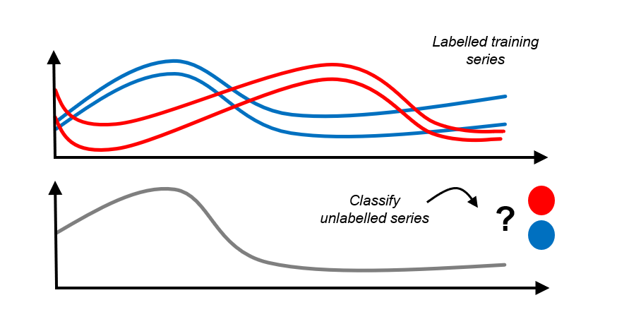
分类 = 在时间序列/类别示例上训练后，尝试为每个时间序列分配一个类别

示例：随时间变化的每日能源消耗曲线 - 预测季节（例如冬季/夏季）或消费者类型

回归 = 在时间序列/类别示例上训练后，尝试为每个时间序列分配一个连续的数值

示例：化学反应器的温度/压力/时间曲线 - 预测总纯度（1 的分数）

聚类 = 将不同的时间序列放入少量相似性桶中

示例：服务级别协议 (SLA) 违规 - 对收集的面板数据进行分组，以识别 SLA 失败的常见原因

时间序列分类

time series classification

[1]:

import numpy as np
import pandas as pd

# Increase display width
pd.set_option("display.width", 1000)

2.1 面板数据 - `sktime` 数据格式#

Panel 是一种抽象数据类型，其中观测值为

instance，例如，患者
variable，例如，患者的血压、体温
time/index，例如，2023 年 1 月 12 日（通常但并非一定是时间索引！）

一个值 X 是：“患者‘A’在 2023 年 1 月 12 日的血压为‘X’”

时间序列分类、回归、聚类：按实例切片 Panel 数据

首选格式 1：具有 2 级 MultiIndex（实例，时间）和列（变量）的 pd.DataFrame

首选格式 2：具有索引（实例，变量，时间）的 3D np.ndarray

sktime 支持并识别多种数据格式，以方便使用和内部使用，例如 dask, xarray
抽象数据类型 = “scitype”；内存规范 = “mtype”
有关内存数据表示和数据加载的更多信息，请参阅教程

2.1.1 首选格式 1 - `pd-multiindex` 规范#

pd-multiindex = 具有 2 级 MultiIndex（实例，时间）和列（变量）的 pd.DataFrame

[2]:

from sktime.datasets import load_italy_power_demand

# load an example time series panel in pd-multiindex mtype
X, _ = load_italy_power_demand(return_type="pd-multiindex")

# renaming columns for illustrative purposes
X.columns = ["total_power_demand"]
X.index.names = ["day_ID", "hour_of_day"]

意大利电力需求数据集包含

1096 个独立时间序列实例 = 总电力需求（减去均值）的单日数据
每个时间序列实例一个变量，total_power_demand
- 该日、该小时内的总电力需求
- 由于只有一个列，这是一个单变量数据集
独立时间序列在 24 个时间（周期）点进行观测（所有实例的数量相同）

在该数据集中，日期是混杂的，范围不同（独立采样）。

被认为是独立的 - 因为一个样本中的 hour_of_day 不影响另一个样本中的 hour_of_day
用于任务，例如，“从模式中识别季节或工作日/周末”

[3]:

[3]:

		total_power_demand
day_ID	hour_of_day
0	0	-0.710518
	1	-1.183320
	2	-1.372442
	3	-1.593083
	4	-1.467002
...	...	...
1095	19	0.180490
	20	-0.094058
	21	0.729587
	22	0.210995
	23	-0.002542

26304 rows × 1 columns

[4]:

from sktime.datasets import load_basic_motions

# load an example time series panel in pd-multiindex mtype
X, _ = load_basic_motions(return_type="pd-multiindex")

# renaming columns for illustrative purposes
X.columns = ["accel_1", "accel_2", "accel_3", "gyro_1", "gyro_2", "gyro_3"]
X.index.names = ["trial_no", "timepoint"]

基本运动数据集包含

80 个独立时间序列实例 = 试验 = 进行跑步、羽毛球等活动的人员
每个时间序列实例六个变量，dim_0 到 dim_5（根据它们代表的值重命名）
- 3 个加速度计测量和 3 个陀螺仪测量
- 因此是一个多变量数据集
独立时间序列在 100 个时间点进行观测（所有实例的数量相同）

[5]:

# The outermost index represents the instance number
# whereas the inner index represents the index of the particular index
# within that instance.
X

[5]:

		accel_1	accel_2	accel_3	gyro_1	gyro_2	gyro_3
trial_no	timepoint
0	0	0.079106	0.394032	0.551444	0.351565	0.023970	0.633883
	1	0.079106	0.394032	0.551444	0.351565	0.023970	0.633883
	2	-0.903497	-3.666397	-0.282844	-0.095881	-0.319605	0.972131
	3	1.116125	-0.656101	0.333118	1.624657	-0.569962	1.209171
	4	1.638200	1.405135	0.393875	1.187864	-0.271664	1.739182
...	...	...	...	...	...	...	...
79	95	28.459024	-16.633770	3.631869	8.978229	-3.611533	-1.491489
	96	10.260094	0.102775	1.269261	-1.645964	-3.377157	1.283746
	97	4.316471	-3.574319	2.063831	-1.717875	-1.843054	0.484734
	98	0.704446	-4.920444	2.851857	-2.982977	-0.809665	-0.721774
	99	-2.074749	-6.892377	4.848379	-1.350330	-1.203844	-1.776470

8000 rows × 6 columns

pandas 提供了一种简单的方法来访问多级索引 DataFrame 中的值范围

[6]:

# Select:
# * the fourth variable (gyroscope 1)
# * of the first instance (trial 1 = 0 in python)
# * values at all 100 timestamps
#
X.loc[0, "gyro_1"]

[6]:

timepoint
0     0.351565
1     0.351565
2    -0.095881
3     1.624657
4     1.187864
        ...
95    0.039951
96   -0.029297
97    0.000000
98    0.000000
99   -0.007990
Name: gyro_1, Length: 100, dtype: float64

或者如果你想访问单个值

[7]:

# Select:
# * the fifth time time point (5 = 4 in python, because of 0-indexing)
# * the third variable (accelerometer 3)
# * of the forty-third instance (trial 43 = 42 in python)

X.loc[(42, 4), "accel_3"]

[7]:

-1.27952

2.1.2 首选格式 2 - `numpy3D` 规范#

numpy3D = 具有索引（实例，变量，时间）的 3D np.ndarray

实例/时间索引被解释为整数

重要：与 pd-multiindex 不同，这假定

所有独立序列具有相同的长度
所有独立序列具有相同的索引

[8]:

from sktime.datasets import load_italy_power_demand

# load an example time series panel in numpy mtype
X, _ = load_italy_power_demand(return_type="numpy3D")

意大利电力需求数据集包含

1096 个独立时间序列实例 = 总电力需求（减去均值）的单日数据
每个时间序列实例一个变量，在 numpy 中未命名
独立时间序列在 24 个时间（周期）点进行观测（所有实例的数量相同）

[9]:

# (num_instances, num_variables, length)
X.shape

[9]:

(1096, 1, 24)

[10]:

from sktime.datasets import load_basic_motions

# load an example time series panel in numpy mtype
X, _ = load_basic_motions(return_type="numpy3D")

基本运动数据集包含

80 个独立时间序列实例 = 试验 = 从事活动（跑步、羽毛球等）的人员
每个时间序列实例六个变量，在 numpy 中未命名
独立时间序列在 100 个时间点进行观测（所有实例的数量相同）

[11]:

X.shape

[11]:

(80, 6, 100)

2.2 时间序列分类、回归、聚类 - 基本示例#

上述任务与 sklearn 中的“表格”分类、回归、聚类非常相似

主要区别

在“表格”分类等任务中，一个（特征）实例是一行特征向量
在 TSC 中，一个（特征）实例是完整的时间序列，长度可能不等，索引集不同

更正式地

“表格”分类
- 训练对 \((x_1, y_1), \dots, (x_n, y_n)\)
  - 其中 \(x_i\) 是 pd.DataFrame 的行（相同列类型）
  - 并且 \(y_i \in \mathcal{C}\)，其中 \(\mathcal{C}\) 是一个有限集
- 用于训练一个分类器，该分类器
  - 对于新的 pd.DataFrame 行 \(x_*\)
  - 预测 \(y_* \in \mathcal{C}\)

时间序列分类
- 训练对 \((x_1, y_1), \dots, (x_n, y_n)\)
  - 其中 \(x_i\) 是来自特定领域的时间序列实例
  - 并且 \(y_i \in \mathcal{C}\)，其中 \(\mathcal{C}\) 是一个有限集
- 用于训练一个分类器，该分类器
  - 对于新的时间序列实例 \(x_*\)
  - 预测 \(y_* \in \mathcal{C}\)

时间序列回归、聚类也非常相似 - 留给读者练习 :-)

sktime 设计启示

需要表示时间序列集合（面板），有关 Panel 数据表示的更多详细信息，请参阅内存数据表示和数据加载教程。
- 与“相邻”学习任务（例如面板预测）中的情况相同
- 与转换估计器相同
使用序列性、可以处理不等长、缺失值等的算法
算法通常基于时间序列之间的距离或核 - 需要在框架中涵盖这一点
但我们可以使用熟悉的 fit / predict 以及 scikit-learn / scikit-base 接口！

2.2.3 时间序列分类 - 部署示例#

TSC 基本部署示例

加载/设置训练数据，X 采用 Panel（更具体地说是 numpy3D）格式，y 采用 1D np.ndarray 格式
加载/设置用于预测的新数据（也可以在第 3 步之后完成）
使用类似 sklearn 的语法指定分类器
将分类器拟合到训练数据，fit(X, y)
在新数据上预测标签，predict(X_new)

[12]:

# steps 1, 2 - prepare osuleaf dataset (train and new)
from sktime.datasets import load_italy_power_demand

X_train, y_train = load_italy_power_demand(split="train", return_type="numpy3D")
X_new, _ = load_italy_power_demand(split="test", return_type="numpy3D")

[13]:

# this is in numpy3D format, but could also be pd-multiindex or other
X_train.shape

[13]:

(67, 1, 24)

[14]:

# y is a 1D np.ndarray of labels - same length as number of instances in X_train
y_train.shape

[14]:

(67,)

[15]:

# step 3 - specify the classifier
from sktime.classification.distance_based import KNeighborsTimeSeriesClassifier

# example 1 - 3-NN with simple dynamic time warping distance (requires numba)
clf = KNeighborsTimeSeriesClassifier(n_neighbors=3)

# example 2 - custom distance:
# 3-nearest neighbour classifier with Euclidean distance (on flattened time series)
# (requires scipy)
from sktime.classification.distance_based import KNeighborsTimeSeriesClassifier
from sktime.dists_kernels import FlatDist, ScipyDist

eucl_dist = FlatDist(ScipyDist())
clf = KNeighborsTimeSeriesClassifier(n_neighbors=3, distance=eucl_dist)

我们可以在这里指定任何 sktime 分类器 - 其余部分保持不变！

[16]:

# all classifiers is scikit-learn / scikit-base compatible!
# nested parameter interface via get_params, set_params
clf.get_params()

[16]:

{'algorithm': 'brute',
 'distance': FlatDist(transformer=ScipyDist()),
 'distance_mtype': None,
 'distance_params': None,
 'leaf_size': 30,
 'n_jobs': None,
 'n_neighbors': 3,
 'pass_train_distances': False,
 'weights': 'uniform',
 'distance__transformer': ScipyDist(),
 'distance__transformer__colalign': 'intersect',
 'distance__transformer__metric': 'euclidean',
 'distance__transformer__metric_kwargs': None,
 'distance__transformer__p': 2,
 'distance__transformer__var_weights': None}

[17]:

# step 4 - fit/train the classifier
clf.fit(X_train, y_train)

[17]:

KNeighborsTimeSeriesClassifier(distance=FlatDist(transformer=ScipyDist()),
                               n_neighbors=3)

请重新运行此单元格以显示 HTML repr 或信任此 notebook。

[18]:

# the classifier is now fitted
clf.is_fitted

[18]:

True

[19]:

# and we can inspect fitted parameters if we like
clf.get_fitted_params()

[19]:

{'classes': array(['1', '2'], dtype='<U1'),
 'fit_time': 369,
 'knn_estimator': KNeighborsClassifier(algorithm='brute', metric='precomputed', n_neighbors=3),
 'n_classes': 2,
 'knn_estimator__classes': array(['1', '2'], dtype='<U1'),
 'knn_estimator__effective_metric': 'precomputed',
 'knn_estimator__effective_metric_params': {},
 'knn_estimator__n_features_in': 67,
 'knn_estimator__n_samples_fit': 67,
 'knn_estimator__outputs_2d': False}

[20]:

# step 5 - predict labels on new data
y_pred = clf.predict(X_new)

[21]:

# y_pred is an 1D np.ndarray, similar to sklearn classification output
y_pred

[21]:

array(['2', '2', '2', ..., '2', '2', '2'], dtype='<U1')

[22]:

# predictions and unique counts, for illustration
unique, counts = np.unique(y_pred, return_counts=True)
unique, counts

[22]:

(array(['1', '2'], dtype='<U1'), array([510, 519], dtype=int64))

在一个单元格中全部完成

[23]:

# steps 1, 2 - prepare osuleaf dataset (train and new)
from sktime.datasets import load_italy_power_demand

X_train, y_train = load_italy_power_demand(split="train", return_type="numpy3D")
X_new, _ = load_italy_power_demand(split="test", return_type="numpy3D")

# step 3 - specify the classifier
from sktime.classification.distance_based import KNeighborsTimeSeriesClassifier
from sktime.dists_kernels import FlatDist, ScipyDist

eucl_dist = FlatDist(ScipyDist())
clf = KNeighborsTimeSeriesClassifier(n_neighbors=3, distance=eucl_dist)

# step 4 - fit/train the classifier
clf.fit(X_train, y_train)

# step 5 - predict labels on new data
y_pred = clf.predict(X_new)

2.2.4 时间序列分类 - 简单评估示例#

评估类似于 sklearn 分类器 - 我们分割数据集并在测试集上评估性能。

这包括以下附加步骤

分割初始历史数据，例如使用 train_test_split
将预测结果与保留的数据集进行比较

[24]:

from sktime.classification.distance_based import KNeighborsTimeSeriesClassifier
from sktime.datasets import load_italy_power_demand

# data should be split into train/test
X_train, y_train = load_italy_power_demand(split="train", return_type="numpy3D")
X_test, y_test = load_italy_power_demand(split="test", return_type="numpy3D")

# step 3-5 are the same

from sktime.dists_kernels import FlatDist, ScipyDist

eucl_dist = FlatDist(ScipyDist())
clf = KNeighborsTimeSeriesClassifier(n_neighbors=3, distance=eucl_dist)

clf.fit(X_train, y_train)
y_pred = clf.predict(X_test)

# for simplest evaluation, compare ground truth to predictions
from sklearn.metrics import accuracy_score

accuracy_score(y_test, y_pred)

[24]:

0.956268221574344

2.2.5 时间序列分类 - 处理多变量数据#

介绍三种处理多变量数据的常用方法

具有原生多变量能力的分类器，例如，TimeSeriesForestClassifier。

带有 capability: multivariate 标签的估计器原生支持多变量 X 输入。有关如何搜索这些估计器，请参阅 2.3 节。

通过 ``IndepDist`` 或 ``CombinedDistance`` 进行距离聚合。

IndepDist 将多个变量上的单变量时间序列距离聚合成一个整体的多变量距离。

在数学上，IndepDist 表示一个多变量距离 \(d_g(x,y)\)，定义为

\[d_g(x,y)=g(d(x_1,y_1),d(x_2,y_2),…,d(x_D,y_D)),\]

其中 \(g\) 是一个选定的聚合函数，如求和、均值或最大值。

通过 ``CombinedDistance`` 进行距离构建。

CombinedDistance 在选择上述函数 \(g\) 方面提供了更大的灵活性，支持任意算术运算。

该类还可以通过使用 dist1 + dist2 等算术运算的便利语法进行调用。

有关自定义时间序列距离或核的更多详细信息，请参阅教程

TimeSeriesForestClassifier 是一个原生处理多变量数据的估计器的很好的例子。

[25]:

from sktime.classification.interval_based import TimeSeriesForestClassifier
from sktime.datasets import load_arrow_head

# step 1-- prepare a dataset (multivariate for demonstration)
X_train, y_train = load_arrow_head(split="train")
X_new, _ = load_arrow_head(split="test")

# step 2-- define the TimeSeriesForestClassifier
tsf = TimeSeriesForestClassifier()

# step 3-- train the classifier on the data
tsf.fit(X_train, y_train)

# step 4-- predict labels on the new data
y_pred = tsf.predict(X_new[:5])

[26]:

y_pred

[26]:

array(['0', '2', '0', '0', '0'], dtype='<U1')

在多变量数据集上使用 sum 聚合函数的 IndepDist 示例。

[27]:

from sktime.classification.distance_based import KNeighborsTimeSeriesClassifier
from sktime.datasets import load_arrow_head
from sktime.dists_kernels.compose_tab_to_panel import FlatDist
from sktime.dists_kernels.indep import IndepDist
from sktime.dists_kernels.scipy_dist import ScipyDist

# step 1-- prepare a dataset (multivariate for demonstrating purposes)
X_train, y_train = load_arrow_head(split="train", return_X_y=True)
X_new, _ = load_arrow_head(split="test", return_X_y=True)

# step 2-- define a classification estimator with distance parameter IndepDist
indep_dist_sum = IndepDist(dist=FlatDist(ScipyDist()), aggfun="sum")
knn_sum = KNeighborsTimeSeriesClassifier(distance=indep_dist_sum)

# step 3-- train the models with the data
knn_sum.fit(X_train, y_train)

# step 4-- predict labels on new data
y_pred = knn_sum.predict(X_new[:5])  # Smaller set for faster runtime.

IndepDist 提供了从多种选择中选择 aggfun 参数的能力 - sum, mean, median, max, min。

[28]:

print("Prediction with sum aggregation: ", y_pred)

Prediction with sum aggregation:  ['0' '0' '0' '0' '0']

下面是使用 CombinedDistance 的另一种实现，它在单独的组件上应用 DtwDist()。

[29]:

from sktime.classification.distance_based import KNeighborsTimeSeriesClassifier
from sktime.datasets import load_arrow_head
from sktime.dists_kernels.algebra import CombinedDistance
from sktime.dists_kernels.compose_tab_to_panel import AggrDist, FlatDist
from sktime.dists_kernels.scipy_dist import ScipyDist

# step 1-- load a dataset
X_train, y_train = load_arrow_head(split="train", return_X_y=True)
X_new, _ = load_arrow_head(split="test", return_X_y=True)

# step 2-- setup combined distance
combined_dist = CombinedDistance([FlatDist(ScipyDist()), AggrDist(ScipyDist())])

## step 3-- initialize the classifier
knn_combined_dist = KNeighborsTimeSeriesClassifier(distance=combined_dist)

## step 4-- train the classifier
knn_combined_dist.fit(X_train, y_train)

## step 5-- obtain the predictions from the classifier.
y_pred = knn_combined_dist.predict(X_new[:5])

[30]:

y_pred

[30]:

array(['0', '0', '0', '0', '0'], dtype='<U1')

2.2.6 时间序列回归 - 基本示例#

TSR 示例与 TSC 完全相同，除了

fit 输入中的 y 和 predict 输出应为浮点型 1D np.ndarray，而不是类别型
其他算法被常用且/或性能良好

[31]:

# steps 1, 2 - prepare dataset (train and new)
from sktime.datasets import load_covid_3month

X_train, y_train = load_covid_3month(split="train")
y_train = y_train.astype("float")
X_new, _ = load_covid_3month(split="test")
X_new = X_new.loc[:2]  # smaller dataset for faster notebook runtime

# step 3 - specify the regressor
from sktime.regression.distance_based import KNeighborsTimeSeriesRegressor

clf = KNeighborsTimeSeriesRegressor(n_neighbors=3, distance=eucl_dist)

# step 4 - fit/train the regressor
clf.fit(X_train, y_train)

# step 5 - predict labels on new data
y_pred = clf.predict(X_new)

[32]:

y_pred  # predictions are array of float

[32]:

array([0.02957762, 0.0065062 , 0.00183655])

2.2.7 时间序列聚类 - 基本示例#

TS 聚类类似 - 第一步也是 fit，但它是无监督的

即，没有标签 y，下一步是检查聚类

[33]:

# step 1 - prepare dataset (train and new)
from sktime.datasets import load_italy_power_demand

X, _ = load_italy_power_demand(split="train", return_type="numpy3D")

# step 2 - specify the clusterer
from sktime.clustering.dbscan import TimeSeriesDBSCAN
from sktime.dists_kernels import FlatDist, ScipyDist

eucl_dist = FlatDist(ScipyDist())
clst = TimeSeriesDBSCAN(distance=eucl_dist, eps=2)

# step 3 - fit the clusterer to the data
clst.fit(X)

# step 4 - inspect the clustering
clst.get_fitted_params()

[33]:

{'core_sample_indices': array([ 0,  1,  3,  4,  6,  7,  8,  9, 10, 11, 12, 13, 14, 16, 17, 18, 19,
        20, 21, 22, 23, 24, 25, 26, 27, 28, 29, 30, 32, 33, 34, 35, 36, 37,
        38, 39, 40, 41, 42, 43, 44, 45, 46, 47, 50, 52, 53, 54, 55, 56, 57,
        58, 60, 61, 62, 63, 64, 65], dtype=int64),
 'dbscan': DBSCAN(eps=2, metric='precomputed'),
 'fit_time': 0,
 'labels': array([ 0,  0, -1,  0,  0,  1,  0,  0,  0,  0,  0,  0,  0,  0,  0,  1,  0,
         0,  0,  0,  0,  0,  0,  0,  0,  0,  0,  0,  0,  0,  0,  1,  0,  0,
         0,  0,  0,  0,  0,  0,  0,  0,  0,  0,  0,  0,  1,  0,  1,  0,  0,
         0,  0,  0,  0,  0,  0,  0,  0, -1,  0,  0,  0,  0,  0,  0, -1],
       dtype=int64),
 'dbscan__components': array([[0.        , 2.21059984, 7.22653506, ..., 2.43397663, 3.42512865,
         5.77701453],
        [2.21059984, 0.        , 7.31863575, ..., 0.8952782 , 2.01224344,
         5.73199202],
        [2.98199582, 1.8413087 , 7.5785501 , ..., 1.5676963 , 1.41086552,
         5.96418696],
        ...,
        [3.78429193, 2.68599227, 6.32367754, ..., 2.71202763, 1.36130647,
         4.47124464],
        [2.43397663, 0.8952782 , 7.59888847, ..., 0.        , 1.98453315,
         5.99830821],
        [3.42512865, 2.01224344, 7.02761342, ..., 1.98453315, 0.        ,
         5.27610504]]),
 'dbscan__core_sample_indices': array([ 0,  1,  3,  4,  6,  7,  8,  9, 10, 11, 12, 13, 14, 16, 17, 18, 19,
        20, 21, 22, 23, 24, 25, 26, 27, 28, 29, 30, 32, 33, 34, 35, 36, 37,
        38, 39, 40, 41, 42, 43, 44, 45, 46, 47, 50, 52, 53, 54, 55, 56, 57,
        58, 60, 61, 62, 63, 64, 65], dtype=int64),
 'dbscan__labels': array([ 0,  0, -1,  0,  0,  1,  0,  0,  0,  0,  0,  0,  0,  0,  0,  1,  0,
         0,  0,  0,  0,  0,  0,  0,  0,  0,  0,  0,  0,  0,  0,  1,  0,  0,
         0,  0,  0,  0,  0,  0,  0,  0,  0,  0,  0,  0,  1,  0,  1,  0,  0,
         0,  0,  0,  0,  0,  0,  0,  0, -1,  0,  0,  0,  0,  0,  0, -1],
       dtype=int64),
 'dbscan__n_features_in': 67}

2.3 搜索估计器、估计器标签#

sktime 中的估计器带有标签。

以“capability”开头的标签指示估计器可以或不能做的事情，例如，

"capability:missing_values" - 处理缺失值
"capability:multivariate" - 处理多变量输入
"capability:unequal_length" - 处理其中独立时间序列长度不等和/或索引不等的时间序列面板

估计器 scitype（例如，分类器、回归器）的所有标签都可以通过 sktime.registry.all_tags 查看

[34]:

from sktime.registry import all_tags

all_tags("classifier", as_dataframe=True)

[34]:

	name	scitype	type	描述
0	X_inner_mtype	estimator	(list, str)	内部 _fit/_pr... 是哪种机器类型
1	作者	object	(list, str)	对象的作者列表，每位作者是一个 G...
2	capability:contractable	estimator	bool	协定时间设置，估计器是否支持...
3	capability:feature_importance	estimator	bool	估计器能否提供特征重要性？
4	capability:missing_values	object	bool	估计器能否处理缺失数据（NA, np....）
5	capability:multioutput	[classifier, regressor]	bool	估计器能否处理多输出时间序列...
6	capability:multithreading	[classifier, early_classifier]	bool	分类器能否设置 n_jobs 以使用多个...
7	capability:multivariate	[classifier, clusterer, early_classifier, para...	bool	估计器能否应用于时间序列...
8	capability:predict_proba	[classifier, clusterer]	bool	估计器是否实现了非默认的 pre...
9	capability:train_estimate	estimator	bool	估计器能否估计其在 ... 上的性能
10	capability:unequal_length	[aligner, classifier, clusterer, early_classif...	bool	估计器能否处理不等长的时间序列...
11	classifier_type	classifier	(list, [dictionary, distance, feature, hybrid,...	分类器属于哪种类型...
12	distribution_type	estimator	str	数据的分布类型（字符串）
13	distribution_type	estimator	str	数据的分布类型（字符串）
14	env_marker	object	str	估计器的环境标记 (PEP 508) 要求...
15	fit_is_empty	estimator	bool	估计器是否有空的 fit 方法？
16	处理缺失数据	estimator	bool	估计器能否处理缺失数据（NA, np....）
17	维护者	object	(list, str)	对象的当前维护者，每位维护者...
18	object_type	object	str	对象类型：估计器、转换器、回归器...
19	python_dependencies	object	(list, str)	估计器的 Python 依赖项（字符串或列表）...
20	python_dependencies_alias	object	dict	用于依赖导入别名的已弃用标签
21	python_version	object	str	估计器的 Python 版本规范（PEP 440）...
22	requires_cython	object	bool	对象是否需要 C 编译器...
23	reserved_params	estimator	(list, str)	基类保留的参数和 pres...
24	sktime_version	object	str	此估计器类来自的 sktime 版本...
25	visual_block_kind	estimator	(str, [single, serial, parallel])	如何显示元估计器的 HTML 表示...
26	y_inner_mtype	estimator	(list, str)	内部 _fit/_pr... 是哪种机器类型

有效的估计器类型列在 all_tags docstring 或 sktime.registry.BASE_CLASS_REGISTER 中

[35]:

from sktime.registry import get_obj_scitype_list

# get only fist table column, the list of types
get_obj_scitype_list()

[35]:

['aligner',
 'classifier',
 'clusterer',
 'detector',
 'early_classifier',
 'estimator',
 'forecaster',
 'global_forecaster',
 'metric',
 'metric_detection',
 'metric_forecasting',
 'metric_forecasting_proba',
 'network',
 'object',
 'param_est',
 'regressor',
 'series-annotator',
 'splitter',
 'transformer',
 'transformer-pairwise',
 'transformer-pairwise-panel',
 'distribution']

要查找特定类型的所有估计器，请使用 sktime.registry.all_estimators 的 filter_tags 参数

[36]:

# list all classifiers in sktime
from sktime.registry import all_estimators

all_estimators("classifier", as_dataframe=True)

C:\Workspace\sktime\sktime\utils\dependencies\_dependencies.py:149: UserWarning: This functionality requires package 'torch' to be present in the python environment, but 'torch' was not found. To install the requirement 'torch', please run: pip install torch`
  _raise_at_severity(msg, severity, caller="_check_soft_dependencies")

[36]:

	name	object
0	Arsenal	<class 'sktime.classification.kernel_based._ar...
1	BOSSEnsemble	<class 'sktime.classification.dictionary_based...
2	BOSSVSClassifierPyts	<class 'sktime.classification.dictionary_based...
3	BaggingClassifier	<class 'sktime.classification.ensemble._baggin...
4	CNNClassifier	<class 'sktime.classification.deep_learning.cn...
...	...	...
58	TimeSeriesForestClassifier	<class 'sktime.classification.interval_based._...
59	TimeSeriesSVC	<class 'sktime.classification.kernel_based._sv...
60	TimeSeriesSVCTslearn	<class 'sktime.classification.kernel_based._sv...
61	WEASEL	<class 'sktime.classification.dictionary_based...
62	WeightedEnsembleClassifier	<class 'sktime.classification.ensemble._weight...

63 rows × 2 columns

要列出具有特定能力的特定类型的所有估计器，请使用 all_estimators 的 filter_tags 参数

[37]:

# list all classifiers in sktime
# that can classify panels of time series containing missing data
from sktime.registry import all_estimators

all_estimators(
    "classifier",
    as_dataframe=True,
    filter_tags={"capability:missing_values": True},
)

[37]:

	name	object
0	BOSSVSClassifierPyts	<class 'sktime.classification.dictionary_based...
1	BaggingClassifier	<class 'sktime.classification.ensemble._baggin...
2	DummyClassifier	<class 'sktime.classification.dummy._dummy.Dum...
3	KNeighborsTimeSeriesClassifier	<class 'sktime.classification.distance_based._...
4	KNeighborsTimeSeriesClassifierPyts	<class 'sktime.classification.distance_based._...
5	MultiplexClassifier	<class 'sktime.classification.compose._multipl...
6	ShapeletLearningClassifierPyts	<class 'sktime.classification.shapelet_based._...
7	SklearnClassifierPipeline	<class 'sktime.classification.compose._pipelin...
8	TSCGridSearchCV	<class 'sktime.classification.model_selection....
9	TimeSeriesSVC	<class 'sktime.classification.kernel_based._sv...
10	WeightedEnsembleClassifier	<class 'sktime.classification.ensemble._weight...

旁注

别担心列表有多短 - 如果有疑问，总是可以通过 Imputer 构建管道

如下一节所示 :-)

2.4 管道、特征提取、调优、组合#

类似于 sklearn 用于“表格”分类、回归等任务的方式，

sktime 提供了一套丰富的工具，用于

通过转换器进行特征提取
将转换器与任何估计器构建管道
通过网格搜索等方法调优单个估计器或管道
使用单个估计器或其他组合构建集成模型

如果使用基于 numpy 的数据 mtype，sktime 也与 sklearn 接口完全互操作

（尽管这将失去对不等长时间序列的支持）

2.4.1 `sktime` 转换器用于特征提取入门#

所有 sktime 转换器都能原生处理面板数据

[38]:

from sktime.datasets import load_italy_power_demand
from sktime.transformations.series.detrend import Detrender

# load some panel data
X, _ = load_italy_power_demand(return_type="pd-multiindex")

# specify a linear detrender
detrender = Detrender()

# detrend X by removing linear trend from each instance
X_detrended = detrender.fit_transform(X)
X_detrended

[38]:

		dim_0
0	0	0.267711
	1	-0.290155
	2	-0.564339
	3	-0.870044
	4	-0.829027
...	...	...
1095	19	-0.425904
	20	-0.781304
	21	-0.038512
	22	-0.637956
	23	-0.932346

26304 rows × 1 columns

对于 TSC、TSR、聚类等面板任务，有两个区别需要注意

序列到序列转换器将单个序列转换为序列，面板转换为面板。例如，上面的实例级去趋势器
序列到原始转换器将单个序列转换为一组表格特征。例如，摘要特征提取器

这两种类型的转换都可以是实例级的

实例级转换仅使用第 i 个序列来转换第 i 个序列。例如，实例级去趋势器
非实例级转换在所有序列上进行训练，以转换第 i 个序列。例如，PCA，整体均值去趋势器

[39]:

# example of a series-to-primitive transformer
from sktime.transformations.series.summarize import SummaryTransformer

# specify summary transformer
summary_trafo = SummaryTransformer()

# extract summary features - one per instance in the panel
X_summaries = summary_trafo.fit_transform(X)
X_summaries

[39]:

	均值	标准差	最小值	最大值	0.1	0.25	0.5	0.75	0.9
0	-1.041667e-09	1.0	-1.593083	1.464375	-1.372442	-0.805078	0.030207	0.936412	1.218518
1	-1.958333e-09	1.0	-1.630917	1.201393	-1.533955	-0.999388	0.384871	0.735720	1.084018
2	-1.775000e-09	1.0	-1.397118	2.349344	-1.003740	-0.741487	-0.132687	0.265374	1.515756
3	-8.541667e-10	1.0	-1.646458	1.344487	-1.476779	-0.898722	0.266022	0.776495	1.039641
4	-3.416667e-09	1.0	-1.620240	1.303502	-1.511644	-0.978061	0.405495	0.692648	1.061249
...	...	...	...	...	...	...	...	...	...
1091	-1.041667e-09	1.0	-1.817799	1.630397	-1.323058	-0.643414	0.081208	0.568453	1.390523
1092	-4.166666e-10	1.0	-1.550077	1.513605	-1.343747	-0.768526	0.075550	0.857101	1.276013
1093	4.166667e-09	1.0	-1.706992	1.052255	-1.498879	-1.139943	0.467669	0.713195	0.993797
1094	1.583333e-09	1.0	-1.673857	2.420163	-0.744173	-0.479768	-0.266538	0.159923	1.550184
1095	3.495833e-09	1.0	-1.680337	1.461716	-1.488154	-0.810934	0.241501	0.645697	1.184117

1096 rows × 9 columns

就像分类器一样，我们可以通过正确的标签搜索任一类型的转换器

"scitype:transform-input" 和 "scitype:transform-output" 定义输入和输出，例如“序列到序列”（两者都是 scitype 字符串）
"scitype:instancewise" 是布尔值，告诉我们转换是否是实例级的

[40]:

# example: looking for all series-to-primitive transformers that are instance-wise
from sktime.registry import all_estimators

all_estimators(
    "transformer",
    as_dataframe=True,
    filter_tags={
        "scitype:transform-input": "Series",
        "scitype:transform-output": "Primitives",
        "scitype:instancewise": True,
    },
)

[40]:

	name	object
0	Catch22	<class 'sktime.transformations.panel.catch22.C...
1	Catch22Wrapper	<class 'sktime.transformations.panel.catch22wr...
2	FittedParamExtractor	<class 'sktime.transformations.panel.summarize...
3	HurstExponentTransformer	<class 'sktime.transformations.series.hurst.Hu...
4	RandomIntervalFeatureExtractor	<class 'sktime.transformations.panel.summarize...
5	RandomIntervals	<class 'sktime.transformations.panel.random_in...
6	RandomShapeletTransform	<class 'sktime.transformations.panel.shapelet_...
7	SignatureMoments	<class 'sktime.transformations.series.signatur...
8	SignatureTransformer	<class 'sktime.transformations.panel.signature...
9	SummaryTransformer	<class 'sktime.transformations.series.summariz...
10	TSFreshFeatureExtractor	<class 'sktime.transformations.panel.tsfresh.T...
11	Tabularizer	<class 'sktime.transformations.panel.reduce.Ta...
12	TimeBinner	<class 'sktime.transformations.panel.reduce.Ti...

有关转换和特征提取的更多详细信息，请参见教程 3，转换器。

其中的所有组合步骤（例如，链接、列子集）都与 sktime 中的所有估计器类型协同工作，包括分类器、回归器、聚类器。

2.4.2 时间序列面板任务的管道#

所有面板估计器都可以通过 * 双下划线方法或 make_pipeline 与 sktime 转换器构建管道。

该管道执行以下操作

在 fit 中：按顺序运行转换器的 fit_transform，然后运行面板估计器的 fit
在 predict 中，按顺序运行已拟合转换器的 transform，然后运行面板估计器的 predict

（逻辑与 sklearn 管道相同）

[41]:

from sktime.classification.distance_based import KNeighborsTimeSeriesClassifier
from sktime.transformations.series.exponent import ExponentTransformer

pipe = ExponentTransformer() * KNeighborsTimeSeriesClassifier()

# this constructs a ClassifierPipeline, which is also a classifier
pipe

[41]:

ClassifierPipeline(classifier=KNeighborsTimeSeriesClassifier(),
                   transformers=[ExponentTransformer()])

请重新运行此单元格以显示 HTML repr 或信任此 notebook。

[42]:

# alternative to construct:
from sktime.pipeline import make_pipeline

pipe = make_pipeline(ExponentTransformer(), KNeighborsTimeSeriesClassifier())

[43]:

from sktime.datasets import load_unit_test

X_train, y_train = load_unit_test(split="TRAIN")
X_test, _ = load_unit_test(split="TEST")

# this is a ClassifierPipeline with the same interface as knn-classifier
# first applies exponent transform, then knn-classifier
pipe.fit(X_train, y_train)

[43]:

ClassifierPipeline(classifier=KNeighborsTimeSeriesClassifier(),
                   transformers=[ExponentTransformer()])

请重新运行此单元格以显示 HTML repr 或信任此 notebook。

sktime 转换器可以与 sklearn 分类器构建管道！

这使得构建“时间序列特征提取然后 sklearn 分类”管道成为可能

[44]:

from sklearn.ensemble import RandomForestClassifier

from sktime.transformations.series.summarize import SummaryTransformer

# specify summary transformer
summary_rf = SummaryTransformer() * RandomForestClassifier()

summary_rf.fit(X_train, y_train)

[44]:

SklearnClassifierPipeline(classifier=RandomForestClassifier(),
                          transformers=[SummaryTransformer()])

请重新运行此单元格以显示 HTML repr 或信任此 notebook。

2.4.3 使用转换器处理不等长或缺失值#

专家提示：可用于构建管道的有用转换器是那些“提升”功能的转换器！

搜索这些转换器标签

"capability:unequal_length:removes" - 确保面板中所有实例之后都具有相同的长度。示例：填充、截断、重采样。
"capability:missing_values:removes" - 从传递给它的数据（例如，序列、面板）中移除所有缺失值。示例：均值插补

[45]:

# all transformers that guarantee that the output is equal length and equal index
from sktime.registry import all_estimators

all_estimators(
    "transformer",
    as_dataframe=True,
    filter_tags={"capability:unequal_length:removes": True},
)

[45]:

	name	object
0	ClearSky	<class 'sktime.transformations.series.clear_sk...
1	IntervalSegmenter	<class 'sktime.transformations.panel.segment.I...
2	PaddingTransformer	<class 'sktime.transformations.panel.padder.Pa...
3	RandomIntervalSegmenter	<class 'sktime.transformations.panel.segment.R...
4	SlopeTransformer	<class 'sktime.transformations.panel.slope.Slo...
5	SubsequenceExtractionTransformer	<class 'sktime.transformations.series.subseque...
6	TimeBinAggregate	<class 'sktime.transformations.series.binning....
7	TruncationTransformer	<class 'sktime.transformations.panel.truncatio...

[46]:

# all transformers that guarantee the output has no missing values
from sktime.registry import all_estimators

all_estimators(
    "transformer",
    as_dataframe=True,
    filter_tags={"capability:missing_values:removes": True},
)

[46]:

	name	object
0	ClearSky	<class 'sktime.transformations.series.clear_sk...
1	ClustererAsTransformer	<class 'sktime.clustering.compose._as_transfor...
2	DetectorAsTransformer	<class 'sktime.detection.compose._as_transform...
3	Imputer	<class 'sktime.transformations.series.impute.I...

次要说明

某些转换器在某些条件下能保证“没有缺失值”，但并非总是如此，例如 TimeBinAggregate

让我们在一个示例中检查标签

[47]:

# list all classifiers in sktime
from sktime.classification.feature_based import SummaryClassifier

no_missing_clf = SummaryClassifier()

no_missing_clf.get_tags()

[47]:

{'python_version': None,
 'python_dependencies': None,
 'env_marker': None,
 'sktime_version': '0.35.0',
 'object_type': 'classifier',
 'X_inner_mtype': 'numpy3D',
 'y_inner_mtype': 'numpy1D',
 'capability:multioutput': False,
 'capability:multivariate': True,
 'capability:unequal_length': False,
 'capability:missing_values': False,
 'capability:train_estimate': False,
 'capability:feature_importance': False,
 'capability:contractable': False,
 'capability:multithreading': True,
 'capability:predict_proba': True,
 'requires_cython': False,
 'authors': ['MatthewMiddlehurst'],
 'maintainers': 'sktime developers',
 'classifier_type': 'feature'}

[48]:

from sktime.transformations.series.impute import Imputer

clf_can_do_missing = Imputer() * SummaryClassifier()

clf_can_do_missing.get_tags()

[48]:

{'python_version': None,
 'python_dependencies': None,
 'env_marker': None,
 'sktime_version': '0.35.0',
 'object_type': 'classifier',
 'X_inner_mtype': 'pd-multiindex',
 'y_inner_mtype': 'numpy1D',
 'capability:multioutput': False,
 'capability:multivariate': True,
 'capability:unequal_length': False,
 'capability:missing_values': True,
 'capability:train_estimate': False,
 'capability:feature_importance': False,
 'capability:contractable': False,
 'capability:multithreading': False,
 'capability:predict_proba': True,
 'requires_cython': False,
 'authors': ['fkiraly'],
 'maintainers': 'sktime developers',
 'visual_block_kind': 'serial'}

2.4.4 调优和模型选择#

sktime 分类器兼容 sklearn 的模型选择和组合工具，同时使用 sktime 数据格式。

只要使用基于 numpy 的格式或按长度/实例索引的格式，这同样适用于网格调优和交叉验证。

[49]:

from sktime.datasets import load_unit_test

X_train, y_train = load_unit_test(split="TRAIN")
X_test, _ = load_unit_test(split="TEST")

使用 sklearn 的 cross_val_score 和 KFold 功能进行交叉验证

[50]:

from sklearn.model_selection import KFold, cross_val_score

from sktime.classification.feature_based import SummaryClassifier

clf = SummaryClassifier()

cross_val_score(clf, X_train, y=y_train, cv=KFold(n_splits=4))

[50]:

array([0.2, 0.8, 0.6, 0.8])

使用 sklearn 的 GridSearchCV 进行参数调优，我们为 K-NN 分类器调优 k 和距离度量

[51]:

from sklearn.model_selection import GridSearchCV

from sktime.classification.distance_based import KNeighborsTimeSeriesClassifier

knn = KNeighborsTimeSeriesClassifier()
param_grid = {"n_neighbors": [1, 5], "distance": ["euclidean", "dtw"]}
parameter_tuning_method = GridSearchCV(knn, param_grid, cv=KFold(n_splits=4))

parameter_tuning_method.fit(X_train, y_train)
y_pred = parameter_tuning_method.predict(X_test)

2.4.5 高级组合备忘单 - AutoML、bagging、集成#

常见的集成模式：BaggingClassifier, WeightedEnsembleClassifier
与 sklearn 分类器、回归器构建块的可组合性仍然适用
AutoML 可以通过将调优与 MultiplexClassifier 或 MultiplexTransformer 相结合来实现

专家提示：使用固定单列子集进行 bagging 可以将单变量分类器转换为多变量分类器！

2.5 附录 - 扩展指南#

sktime 旨在易于扩展，既可以直接贡献到 sktime，也可以通过自定义方法进行本地/私有扩展。

要使用新的本地或贡献的估计器扩展 sktime，一个好的工作流程是

找到您想添加的估计器类型的正确扩展模板 - 例如，分类器、回归器、聚类器等。扩展模板位于 `extension_templates` 目录中
通读扩展模板 - 这是一个带有 todo 块的 python 文件，这些块标记了需要添加更改的地方。
可选地，如果您计划对接口进行任何重大修改：查看基类 - 请注意，“普通”扩展（例如，新算法）应该在没有此操作的情况下轻松完成。
将扩展模板复制到您自己仓库的本地文件夹（本地/私有扩展），或复制到 sktime 或关联仓库的克隆中（如果是贡献的扩展）的合适位置，放在 sktime.[name_of_task] 目录下；重命名文件并相应地更新文件 docstring。
处理“todo”部分。通常这意味着：更改类名、设置标签值、指定超参数、填写 __init__, _fit, _predict 和/或其他方法（详细信息请参阅扩展模板）。只要不覆盖默认的公共接口，您可以添加私有方法。更多详细信息，请参阅扩展模板。
手动测试您的估计器：导入您的估计器并在上面的基本示例中运行它。
自动测试您的估计器：在您的估计器上调用 sktime.tests.test_all_estimators.check_estimator。您可以在类或对象实例上调用此方法。确保您已根据扩展模板在 get_test_params 方法中指定了测试参数。

如果直接贡献到 sktime 或其关联包，此外

通过 "authors" 和 "maintainers" 标签，将自己添加为新估计器文件（一个或多个）的作者和/或维护者。
创建一个拉取请求，其中仅包含新的估计器（如果不是单个类，还包含其继承树）以及上述的自动化测试。
在拉取请求中，描述该估计器，并最好提供一份关于其实现策略的出版物或其他技术参考。
在创建拉取请求之前，请确保您拥有所有必需的权限，可以将代码贡献给一个宽松许可 (BSD-3) 的开源项目。

使用 nbsphinx 生成。Jupyter notebook 可在此处找到此处。

时间序列分类、回归、聚类及更多#

本 Notebook 概述#

2.1 面板数据 - sktime 数据格式#

2.1.1 首选格式 1 - pd-multiindex 规范#

2.1.2 首选格式 2 - numpy3D 规范#

2.2 时间序列分类、回归、聚类 - 基本示例#

2.2.3 时间序列分类 - 部署示例#

2.2.4 时间序列分类 - 简单评估示例#

2.2.5 时间序列分类 - 处理多变量数据#

2.2.6 时间序列回归 - 基本示例#

2.2.7 时间序列聚类 - 基本示例#

2.3 搜索估计器、估计器标签#

2.4 管道、特征提取、调优、组合#

2.4.1 sktime 转换器用于特征提取入门#

2.4.2 时间序列面板任务的管道#

2.4.3 使用转换器处理不等长或缺失值#

2.4.4 调优和模型选择#

2.4.5 高级组合备忘单 - AutoML、bagging、集成#

2.5 附录 - 扩展指南#

2.1 面板数据 - `sktime` 数据格式#

2.1.1 首选格式 1 - `pd-multiindex` 规范#

2.1.2 首选格式 2 - `numpy3D` 规范#

2.4.1 `sktime` 转换器用于特征提取入门#