![]()
练习#
![]()
[1]:
# !pip install cointanalysis matplotlib numpy pandas pandas_datareader scipy seaborn sklearn statsmodels  # noqa: E501
# !pip install fracdiff
[2]:
import matplotlib.pyplot as plt
import numpy as np
import pandas as pd
import pandas_datareader
import seaborn
from fracdiff import Fracdiff, FracdiffStat, fdiff
from statsmodels.tsa.stattools import adfuller

seaborn.set_style("white")
[3]:
def adf_test(array):
    """Carry out ADF unit-root test and print the result."""
    adf, pvalue, _, _, _, _ = adfuller(array)
    print(f"* ADF statistics: {adf:.3f}")
    print(f"* ADF p-value: {pvalue:.3f}")
5.1#
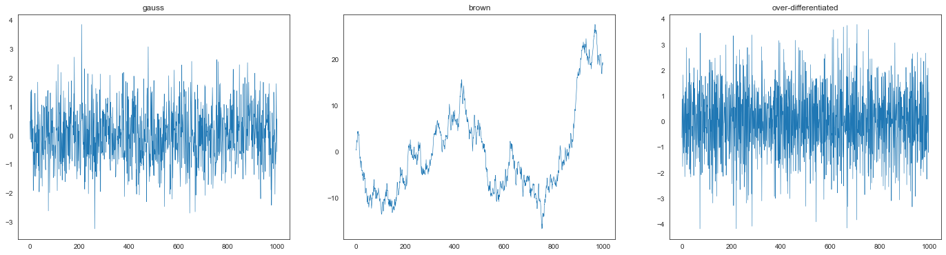
准备高斯分布、其累积和及其微分。
[4]:
np.random.seed(42)
gauss = np.random.randn(1000)
brown = gauss.cumsum()
overd = np.diff(gauss)
[5]:
plt.figure(figsize=(24, 6))

plt.subplot(1, 3, 1)
plt.plot(gauss, lw=0.6)
plt.title("gauss")

plt.subplot(1, 3, 2)
plt.plot(brown, lw=0.6)
plt.title("brown")

plt.subplot(1, 3, 3)
plt.plot(overd, lw=0.6)
plt.title("over-differentiated")

plt.show()
5.1 (a)#
[6]:
adf_test(gauss)
* ADF statistics: -31.811
* ADF p-value: 0.000
5.1 (b)#
累积和的积分阶数为 1。
[7]:
adf_test(brown)
* ADF statistics: -0.966
* ADF p-value: 0.765
5.1 (c)#
过度微分过程的 ADF 统计量和 p 值为
[8]:
adf_test(overd)
* ADF statistics: -11.486
* ADF p-value: 0.000
5.2#
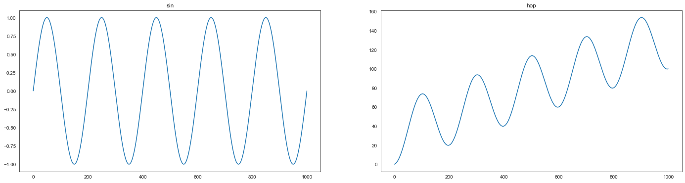
准备
sin函数以及由(sin + shift).cumsum()给出的过程(我们称之为hop)
[9]:
sin = np.sin(np.linspace(0, 10 * np.pi, 1000))
hop = (sin + 0.1).cumsum()
[10]:
plt.figure(figsize=(24, 6))

plt.subplot(1, 2, 1)
plt.title("sin")
plt.plot(sin)

plt.subplot(1, 2, 2)
plt.title("hop")
plt.plot(hop)

plt.show()
5.2 (a)#
[11]:
adf_test(sin)
* ADF statistics: -13323341825676.293
* ADF p-value: 0.000
5.2 (b)#
[12]:
adf_test(hop)
* ADF statistics: -0.284
* ADF p-value: 0.928
让我们看看
hop在不同阶数下的 fracdiff 的 ADF p 值注意:我们将使用固定窗口方法而不是扩展窗口方法。
[13]:
ds = (
    0.200,
    0.400,
    0.600,
    0.800,
    0.900,
    0.990,
    0.999,
    1.000,
)
window = 100

X = hop.reshape(-1, 1)

plt.figure(figsize=(24, 8))
for i, d in enumerate(ds):
    diff = fdiff(hop, d, window=window)
    _, pvalue, _, _, _, _ = adfuller(diff)

    plt.subplot(2, 4, i + 1)
    plt.title(f"hop, {d:.3f} th diff (p={pvalue:.2f})")
    plt.plot(diff)
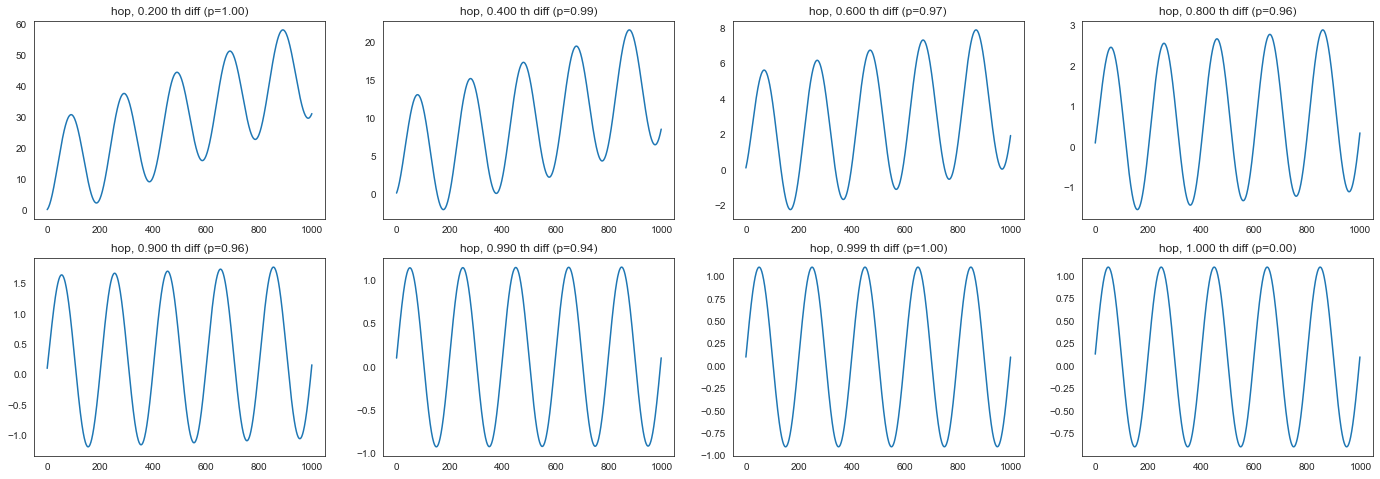
似乎最小阶数非常接近
1.0。让我们使用
FracdiffStat搜索最小值。
[14]:
precision = 10e-8

f = FracdiffStat(window=window, mode="valid", precision=precision, lower=0.9)

diff = f.fit_transform(X)

print(f"* Order: {f.d_[0]:.8f}")
adf_test(diff)
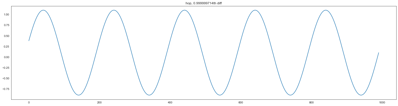
* Order: 0.99999971
* ADF statistics: -280803737.580
* ADF p-value: 0.000
[16]:
# Check

diff = Fracdiff(f.d_[0] - precision, mode="valid").fit_transform(X)

print(f"* Order: {f.d_[0] - precision:.8f}")
adf_test(diff)
* Order: 0.99999961
* ADF statistics: 0.001
* ADF p-value: 0.959
微分后的时间序列看起来像这样
[17]:
plt.figure(figsize=(24, 6))
plt.plot(diff)
plt.title(f"hop, {f.d_[0]:.9f}th diff")
plt.show()
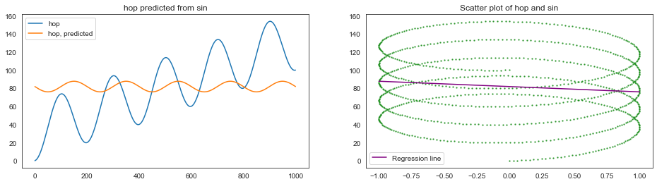
5.3#
5.3 (a)#
[18]:
from sklearn.linear_model import LinearRegression
[19]:
linreg = LinearRegression()
linreg.fit(sin.reshape(-1, 1), hop)

print(f"* R-squared: {linreg.score(sin.reshape(-1, 1), hop):.4f}")
* R-squared: 0.0128
[20]:
plt.figure(figsize=(16, 4))

plt.subplot(1, 2, 1)
plt.title("hop predicted from sin")
plt.plot(hop, label="hop")
plt.plot(linreg.predict(sin.reshape(-1, 1)), label="hop, predicted")
plt.legend()

plt.subplot(1, 2, 2)
plt.title("Scatter plot of hop and sin")
x = np.linspace(-1, 1, 2)
y = linreg.predict(x.reshape(-1, 1))
plt.scatter(sin, hop, s=2, alpha=0.6, color="green")
plt.plot(x, y, color="purple", label="Regression line")
plt.legend()

plt.show()
5.3 (b)#
[21]:
hopd = np.diff(hop)

linreg = LinearRegression()
linreg.fit(sin[1:].reshape(-1, 1), hopd)

print(f"* Coefficient: {linreg.coef_[0]}")
print(f"* Intercept: {linreg.intercept_}")
print(f"* R-squared: {linreg.score(sin[1:].reshape(-1, 1), hopd):.4f}")
* Coefficient: 0.9999999999999994
* Intercept: 0.1
* R-squared: 1.0000
5.3 (c)#
d=1。因为hop的一阶微分是sin加上一个常数。
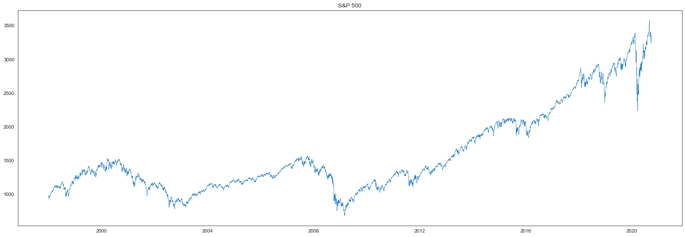
5.4#
注意:我们将使用时间柱(time-bar)而不是美元柱(dollar-bar)。
[22]:
def fetch_spx(begin="1998-01-01", end="2020-09-30"):  # noqa: D103
    return pandas_datareader.data.DataReader("^GSPC", "yahoo", begin, end)["Adj Close"]
[23]:
spx = fetch_spx()
[24]:
plt.figure(figsize=(24, 8))
plt.plot(spx, linewidth=0.6)
plt.title("S&P 500")
plt.show()
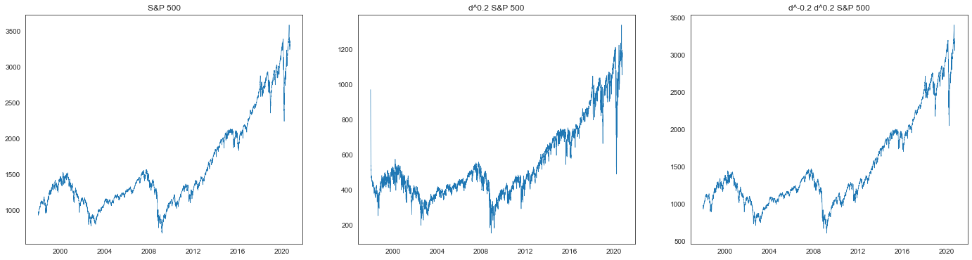
[25]:
d = 0.2
window = 100

d0 = fdiff(spx.values, d, window=window, mode="full")
d1 = fdiff(d0, -d, window=window, mode="full")

spxd = pd.Series(d0, index=spx.index)
spxi = pd.Series(d1, index=spx.index)
原则上,我们得到的是原始时间序列加上一些常数。
同时,由于有限窗口截断系数序列,会产生小的数值误差。
[26]:
plt.figure(figsize=(24, 6))

plt.subplot(1, 3, 1)
plt.title("S&P 500")
plt.plot(spx, linewidth=0.6)

plt.subplot(1, 3, 2)
plt.title(f"d^{d} S&P 500")
plt.plot(spxd, linewidth=0.6)

plt.subplot(1, 3, 3)
plt.title(f"d^{-d} d^{d} S&P 500")
plt.plot(spxi, linewidth=0.6)

plt.show()
5.5#
5.5 (a)#
[27]:
spxlog = spx.apply(np.log)

spxlogcumsum = spxlog.cumsum()
spxlogcumsum
[27]:
Date
1997-12-31        6.877739
1998-01-02       13.760218
1998-01-05       20.644776
1998-01-06       27.518540
1998-01-07       34.389631
                  ...
2020-09-24    41792.094032
2020-09-25    41800.195243
2020-09-28    41808.312436
2020-09-29    41816.424805
2020-09-30    41824.545394
Name: Adj Close, Length: 5725, dtype: float64
5.5 (b)#
[28]:
from fracdiff.tol import window_from_tol_coef

window = window_from_tol_coef(0.5, 1e-5)
window
[28]:
928
[29]:
X = np.array(spxlogcumsum).reshape(-1, 1)

f = FracdiffStat(window=window, mode="valid", upper=2)
diff = f.fit_transform(X)

print(f"* Order: {f.d_[0]:.2f}")
* Order: 1.73
[30]:
# Check stationarity
adf_test(diff)
* ADF statistics: -2.868
* ADF p-value: 0.049
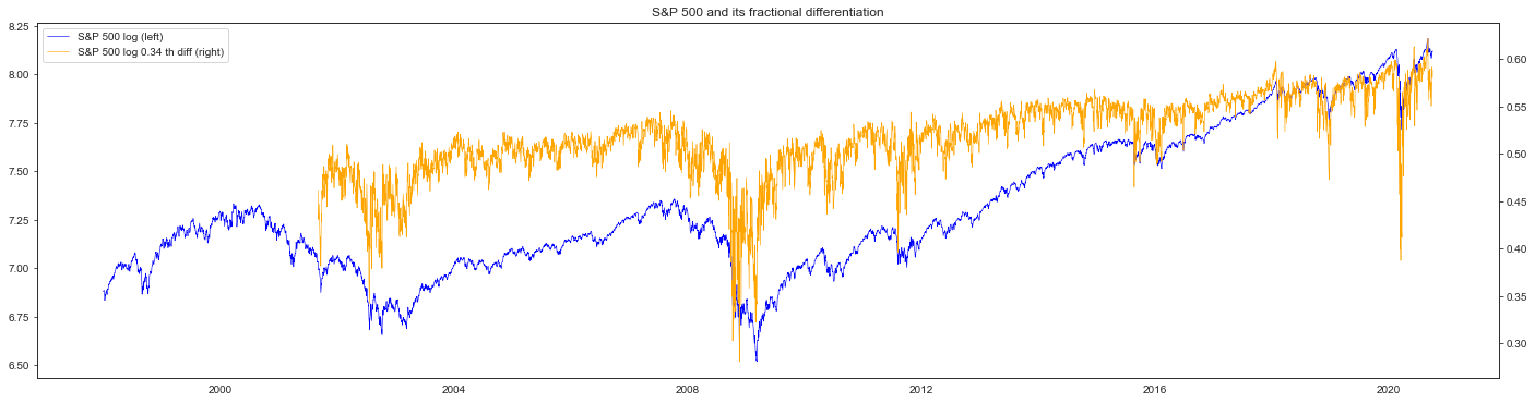
5.5 (c)#
[31]:
X = spxlog.values.reshape(-1, 1)

f = FracdiffStat(window=window, mode="valid")
spxlogd = pd.Series(f.fit_transform(X).reshape(-1), index=spx.index[-diff.size :])
[32]:
corr = np.corrcoef(spxlog[-spxd.size :], spxd)[0, 1]

print(f"* Correlation: {corr:.2f}")
* Correlation: 0.98
[33]:
fig, ax_s = plt.subplots(figsize=(24, 6))
ax_d = ax_s.twinx()

plot_s = ax_s.plot(
    spxlog[-spxd.size :], color="blue", linewidth=0.6, label="S&P 500 log (left)"
)
plot_d = ax_d.plot(
    spxlogd,
    color="orange",
    linewidth=0.6,
    label=f"S&P 500 log {f.d_[0]:.2f} th diff (right)",
)
plots = plot_s + plot_d

plt.title("S&P 500 and its fractional differentiation")
ax_s.legend(plots, [p.get_label() for p in plots], loc=0)

plt.show()
5.5 (d)#
[34]:
from cointanalysis import CointAnalysis
讨论
Xd的协整(cointegration)是没有意义的,因为协整定义在非平稳过程之间,而Xd是平稳的。因此,我们将转而讨论 1.3 阶微分后的时间序列(非平稳)与原始时间序列之间的协整。
[35]:
d = 0.30

# Check non-stationarity
diff = fdiff(spxlog, d, window=window, mode="valid")
spxlogd = pd.Series(diff, index=spxlog.index[-diff.size :])
adf_test(diff)
* ADF statistics: -2.445
* ADF p-value: 0.129
[36]:
pair = np.stack((spxlog[-diff.size :], diff), 1)

ca = CointAnalysis().test(pair)

print(f"* AEG statistics: {ca.stat_:.2f}")
print(f"* AEG p-value: {ca.pvalue_:.2e}")
* AEG statistics: -4.26
* AEG p-value: 2.96e-03
它们是协整的。
大致原因:对于
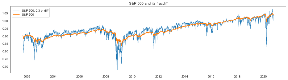
d=0,两个序列完全相同,因此 trivially 协整。对于接近使 fracdiff 平稳的最小值的d,可以通过将原始序列乘以一个无穷小的系数加到 fracdiff 来得到一个几乎平稳的序列。假设插值,可以预期任何介于两者之间的d都会协整。
[37]:
ca.fit(pair)

ys = (-spxlog * ca.coef_[0])[-spxlogd.size :]
yd = spxlogd * ca.coef_[1] - ca.mean_
[38]:
plt.figure(figsize=(16, 4))

plt.plot(yd, linewidth=0.4, label=f"S&P 500, {d} th diff")
plt.plot(ys, linewidth=1.6, label="S&P 500")

plt.legend()
plt.title("S&P 500 and its fracdiff")
plt.show()
[39]:
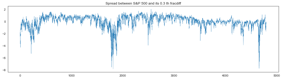
spread = ca.transform(pair)
[40]:
plt.figure(figsize=(16, 4))
plt.plot(spread, linewidth=0.4)
plt.title(f"Spread between S&P 500 and its {d} th fracdiff")
plt.show()
5.5 (e)#
[41]:
from statsmodels.stats.stattools import jarque_bera
[42]:
spxlogd.values.reshape(-1, 1).shape
[42]:
(4798, 1)
[43]:
X = spxlog.values.reshape(-1, 1)

f = FracdiffStat(window=window, mode="valid")
spxlogd = pd.Series(f.fit_transform(X).reshape(-1), index=spx.index[-diff.size :])

spxlr = spxlog.diff()[-spxlogd.size :]  # logreturn

pd.DataFrame(
    {
        "S&P 500": jarque_bera(spx[-spxlogd.size :]),
        "S&P 500 fracdiff": jarque_bera(spxlogd),
        "S&P 500 logreturn": jarque_bera(spxlr),
    },
    index=["JB statistics", "p-value", "skew", "kurtosis"],
).round(3)
[43]:
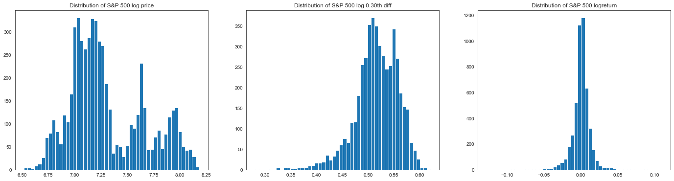
| S&P 500 | S&P 500 fracdiff | S&P 500 对数收益 | |
|---|---|---|---|
| JB 统计量 | 637.418 | 1110.285 | 29941.995 |
| p 值 | 0.000 | 0.000 | 0.000 |
| 偏度 | 0.873 | -0.834 | -0.445 |
| 峰度 | 2.629 | 4.664 | 15.206 |
[44]:
plt.figure(figsize=(24, 6))

plt.subplot(1, 3, 1)
plt.title("Distribution of S&P 500 log price")
plt.hist(spxlog, bins=50)

plt.subplot(1, 3, 2)
plt.title(f"Distribution of S&P 500 log {d:.2f}th diff")
plt.hist(spxlogd, bins=50)

plt.subplot(1, 3, 3)
plt.title("Distribution of S&P 500 logreturn")
plt.hist(spxlr, bins=50)

plt.show()
[ ]: