距离

在本 Notebook 中，我们将使用 sktime 计算时间序列距离

预备知识

import matplotlib.pyplot as plt
import numpy as np

from sktime.datasets import load_macroeconomic
from sktime.distances import distance

距离

距离计算的目标是衡量时间序列 ‘x’ 和 ‘y’ 之间的相似性。距离函数应以 x 和 y 为参数，并返回一个浮点数，该浮点数是计算出的 x 和 y 之间的距离。当时间序列完全相同时，返回的值应为 0.0；当它们不同时，返回一个大于 0.0 的值，该值衡量它们之间的距离。

以下是两个时间序列

X = load_macroeconomic()
country_d, country_c, country_b, country_a = np.split(X["realgdp"].to_numpy()[3:], 4)

plt.plot(country_a, label="County D")
plt.plot(country_b, label="Country C")
plt.plot(country_c, label="Country B")
plt.plot(country_d, label="Country A")
plt.xlabel("Quarters from 1959")
plt.ylabel("Gdp")
plt.legend()

<matplotlib.legend.Legend at 0x7ffa8b8beaf0>

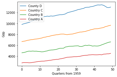
上图展示了一个虚构的场景，比较了四个国家（国家 A、B、C 和 D）自 1959 年以来按季度的 GDP 增长情况。如果我们的任务是确定国家 C 与其他国家有多大差异，一种方法是衡量每个国家之间的距离。

现在将概述如何使用距离模块执行此类任务。

距离模块

要开始使用距离模块，我们需要至少两个时间序列 x 和 y，并且它们必须是 numpy 数组。上面我们已经确定了在此示例中将使用的各种时间序列，分别为 country_a、country_b、country_c 和 country_d。要计算 x 和 y 之间的距离，我们可以使用欧氏距离，如下所示

# Simple euclidean distance
distance(country_a, country_b, metric="euclidean")

27014.721294922445

如上所示，计算 country_a 和 country_b 之间的距离，返回一个浮点数，表示它们的相似性（距离）。我们可以再次执行相同的操作，比较 country_d 与 country_a 的距离

distance(country_a, country_d, metric="euclidean")

58340.14674572803

现在我们可以比较距离计算的结果，我们发现 country_a 比 country_d 更接近 country_b (27014.7 < 58340.1)。

我们可以通过查看上面的图表进一步证实这个结果，看到绿线 (country_b) 比橙线 (country d) 更接近红线 (country_a)。

不同的度量参数

上面我们使用了“欧氏”度量。虽然欧氏距离适用于上面这样的简单示例，但当时间序列更大更复杂时（特别是多元时间序列），它已被证明是不够的。虽然这里不会描述各种不同距离的优点（有关每种距离的描述，请参阅文档），但已经实现了大量专门的时间序列距离，以在距离计算中获得更好的准确性。这些距离包括：‘euclidean’、‘squared’、‘dtw’、‘ddtw’、‘wdtw’、‘wddtw’、‘lcss’、‘edr’、‘erp’

上面列出的所有距离都可以用作度量参数。现在将进行演示

print("Euclidean distance: ", distance(country_a, country_d, metric="euclidean"))
print("Squared euclidean distance: ", distance(country_a, country_d, metric="squared"))
print("Dynamic time warping distance: ", distance(country_a, country_d, metric="dtw"))
print(
    "Derivative dynamic time warping distance: ",
    distance(country_a, country_d, metric="ddtw"),
)
print(
    "Weighted dynamic time warping distance: ",
    distance(country_a, country_d, metric="wdtw"),
)
print(
    "Weighted derivative dynamic time warping distance: ",
    distance(country_a, country_d, metric="wddtw"),
)
print(
    "Longest common subsequence distance: ",
    distance(country_a, country_d, metric="lcss"),
)
print(
    "Edit distance for real sequences distance: ",
    distance(country_a, country_d, metric="edr"),
)
print(
    "Edit distance for real penalty distance: ",
    distance(country_a, country_d, metric="erp"),
)

Euclidean distance:  58340.14674572803
Squared euclidean distance:  3403572722.3130813
Dynamic time warping distance:  3403572722.3130813
Derivative dynamic time warping distance:  175072.58701887555
Weighted dynamic time warping distance:  1701786361.1565406
Weighted derivative dynamic time warping distance:  87536.29350943778
Longest common subsequence distance:  1.0
Edit distance for real sequences distance:  1.0
Edit distance for real penalty distance:  411654.25899999996

虽然上面许多距离的核心都使用了欧氏距离，但它们改变了使用方式，以解决我们在时间序列数据中遇到的各种问题，例如：对齐、相位、形状、维度等。正如所提到的，有关如何最好地使用每种距离及其作用的具体细节，请参阅该距离的文档。

距离的自定义参数

此外，每种距离都有一组不同的参数。现在将使用“dtw”示例概述如何将这些参数传递给“distance”函数。如前所述，有关每种距离的具体参数，请参阅文档。Dtw 是一种 O(n^2) 算法，因此优化该算法一直是重点。一种提高性能的建议是通过在寻找对齐时限制要考虑的值来限制潜在的对齐路径。虽然已经提出了许多边界算法，但最受欢迎的两种是 Sakoe-Chiba 边界或 Itakura 平行四边形边界。现在将使用 LowerBounding 类简要概述这两种方法的工作原理

from sktime.distances import LowerBounding

x = np.zeros((6, 6))
y = np.zeros((6, 6))  # Create dummy data to show the matrix

LowerBounding.NO_BOUNDING.create_bounding_matrix(x, y)

array([[0., 0., 0., 0., 0., 0.],
       [0., 0., 0., 0., 0., 0.],
       [0., 0., 0., 0., 0., 0.],
       [0., 0., 0., 0., 0., 0.],
       [0., 0., 0., 0., 0., 0.],
       [0., 0., 0., 0., 0., 0.]])

上图展示了一个矩阵，该矩阵将“x”中的每个索引映射到“y”中的每个索引。没有边界的 Dtw 会考虑所有这些索引（我们定义为有限值 (0.0) 的边界内的索引）。但是，我们可以使用 Sakoe-Chiba 边界更改被考虑的索引，如下所示

LowerBounding.SAKOE_CHIBA.create_bounding_matrix(x, y, sakoe_chiba_window_radius=0.5)

array([[ 0.,  0.,  0.,  0., inf, inf],
       [ 0.,  0.,  0.,  0.,  0., inf],
       [ 0.,  0.,  0.,  0.,  0.,  0.],
       [ 0.,  0.,  0.,  0.,  0.,  0.],
       [inf,  0.,  0.,  0.,  0.,  0.],
       [inf, inf,  0.,  0.,  0.,  0.]])

生成的矩阵遵循与无边界相同的概念，其中 x 和 y 之间的每个索引都被赋予一个值。如果该值为有限值 (0.0)，则被视为在边界内；如果为无穷大，则被视为在边界外。使用窗口半径为 1 的 Sakoe-Chiba 边界矩阵，我们可以看到得到一条从 0,0 到 5,5 的对角线，其中窗口内的值为 0.0，窗口外的值为无穷大。这减少了 dtw 的计算时间，因为我们考虑的潜在索引减少了 12 个（12 个值是无穷大）。如前所述，还有其他边界技术在矩阵上使用不同的“形状”，例如 Itakura 平行四边形，顾名思义，它在矩阵上产生一个平行四边形形状。

LowerBounding.ITAKURA_PARALLELOGRAM.create_bounding_matrix(x, y, itakura_max_slope=0.3)

array([[ 0.,  0., inf, inf, inf, inf],
       [inf,  0.,  0.,  0., inf, inf],
       [inf,  0.,  0.,  0., inf, inf],
       [inf, inf,  0.,  0.,  0., inf],
       [inf, inf,  0.,  0.,  0., inf],
       [inf, inf,  0.,  0.,  0.,  0.]])

在对边界算法及其使用原因有了基本介绍之后，如何在我们的距离计算中使用它呢？有两种方法

# Create two random unaligned time series to better illustrate the difference

rng = np.random.RandomState(42)
n_timestamps, n_features = 10, 19
x = rng.randn(n_timestamps, n_features)
y = rng.randn(n_timestamps, n_features)

# First we can specify the bounding matrix to use either via enum or int (see
# documentation for potential values):
print(
    "Dynamic time warping distance with Sakoe-Chiba: ",
    distance(x, y, metric="dtw", lower_bounding=LowerBounding.SAKOE_CHIBA, window=1.0),
)  # Sakoe chiba
print(
    "Dynamic time warping distance with Itakura parallelogram: ",
    distance(x, y, metric="dtw", lower_bounding=2, itakura_max_slope=0.2),
)  # Itakura parallelogram using int to specify
print(
    "Dynamic time warping distance with Sakoe-Chiba: ",
    distance(x, y, metric="dtw", lower_bounding=LowerBounding.NO_BOUNDING),
)  # No bounding

Dynamic time warping distance with Sakoe-Chiba:  364.7412646456549
Dynamic time warping distance with Itakura parallelogram:  389.3428989579974
Dynamic time warping distance with Sakoe-Chiba:  364.7412646456549

---

使用 nbsphinx 生成。Jupyter notebook 可在此处找到。